The Persistence of Stock-Selection Residuals
A point-in-time, holdings-based decomposition of mutual fund performance.
Conrad Gann · Blue Water Macro Corp / RiskModels.org · conrad@bwmacro.com · Working paper · v1.5 · June 2026
Revised v1.5 (June 2026): Section 4 numbers re-run on the gated v4 production decomposition (the position-level size/value "stock_specific" cascade) over the 256-fund SPY-benchmarked diversified cohort (extended from 220 via an intensive recovery of pre-2019 N-Q holdings). The finding is unchanged in substance and slightly strengthens on the gated data — the forward top-minus-bottom-quintile stock-selection spread is +2.3pp at t ≈ 3.4 (prior revision +2.4pp / t ≈ 3.0); style and sector controls still do not persist. Full revision history lives in the paper metadata.
Abstract
We define mutual-fund stock-selection skill not as a human trait but as a measurable residual: the idiosyncratic component of performance that remains after the replicable exposures modeled in this decomposition — market, sector, subsector, and Fama–French size/value — are orthogonalized away, and that exhibits cross-sectional stability under out-of-sample testing. Using a point-in-time, holdings-based architecture, we reconstruct each fund's return from the securities it actually held and strip those exposures sequentially — a position-level identification that asks whether the stock-specific return a fund generated persists, not whether a historical return intercept does.
The isolated stock-selection residual exhibits statistically significant out-of-sample persistence: the forward top-minus-bottom-quintile spread is about +2.3 percentage points, with annual non-overlapping reliability of t ≈ 3.4. When the identical point-in-time machinery is applied to style- and sector-timing components as negative-control signals, their forward predictive content does not survive; stock selection does. The differential survival supports the interpretation that the result is specific to the stock-selection residual, not a generic consequence of the validation machinery. The practical consequence is for manager diligence: conventional tools — style classification, sector allocation, benchmark-relative attribution, and recent performance — describe what a fund owned but are weak evidence of repeatable skill, because the standard toolkit blends stock selection with style and sector exposure rather than isolating it. A longitudinal variance decomposition localizes the persistence entirely within the between-fund variance — a persistent between-fund level difference, not a transient timing signal. We read the result narrowly: a robust ranking signal within a chosen mandate, not unconditional evidence that active management outperforms net of fees.
Keywords. mutual fund manager selection · holdings-based return attribution · performance persistence · factor and sector neutralization · active management. JEL: G11, G17, G23.
Contents. (1) What a fund's own documents reveal · (2) What its holdings reveal: a holdings-based, position-level decomposition · (3) The point-in-time testing framework · (4) What persists — and what does not · (5) Ranking managers on the residual that persists · (6) How the industry evaluates managers · (7) Implications for allocators · Appendix A (methodology) · Sources.
Key findings & allocator implications
- Skill, defined as a residual. Stock-selection skill is the idiosyncratic residual that survives orthogonalizing away the replicable exposures modeled here — market, sector, subsector, and Fama–French size/value — from a fund's point-in-time holdings, and that is cross-sectionally stable out of sample. The measurement architecture is the contribution; the persistence is what it finds.
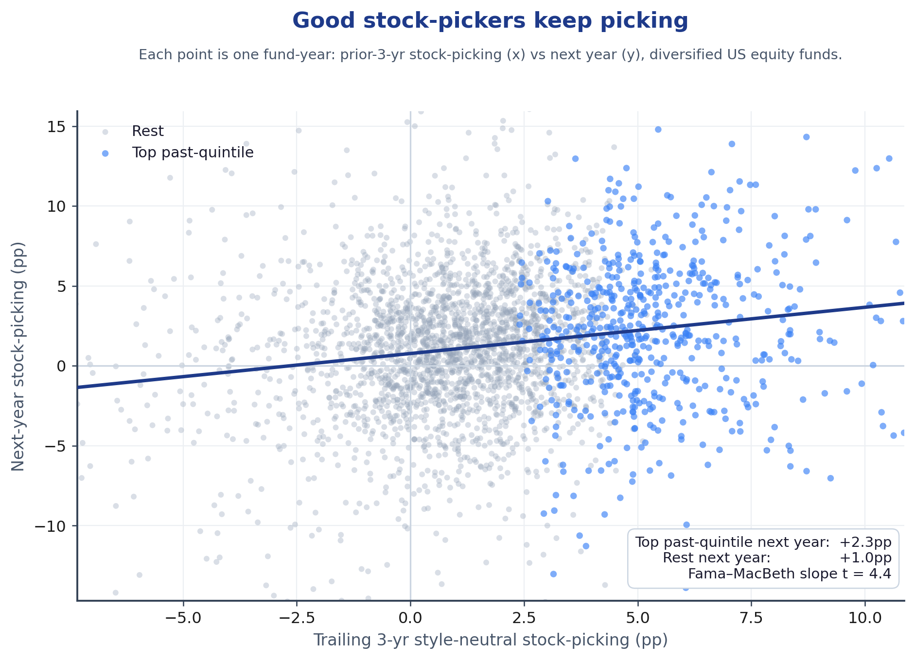
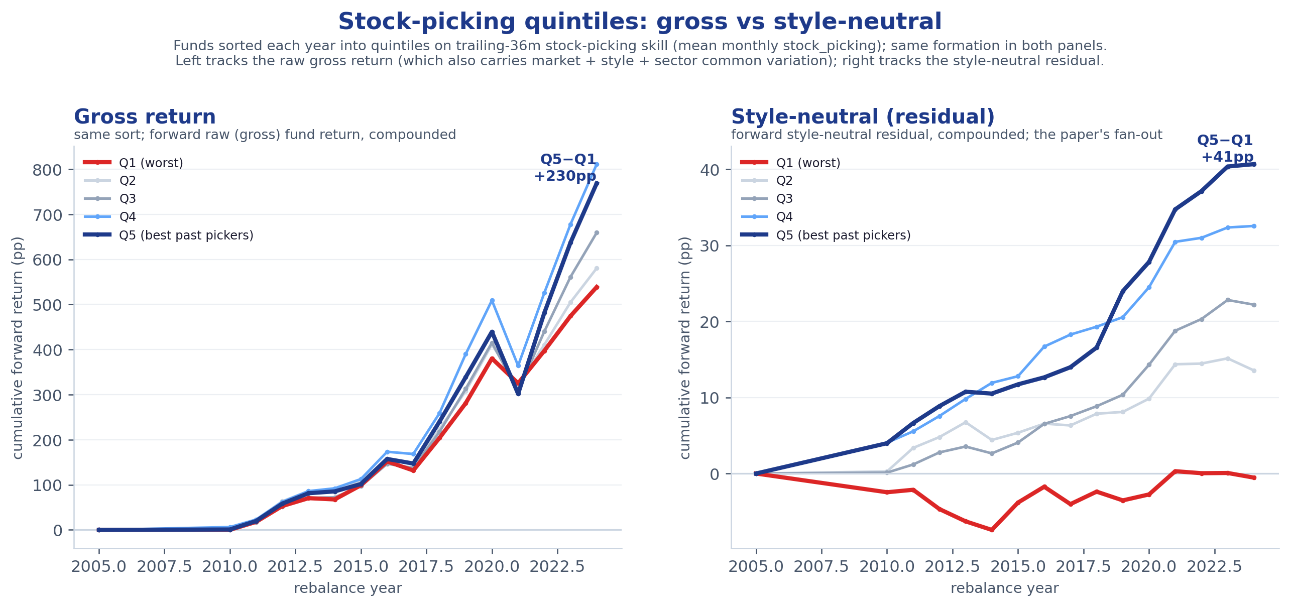
- The number. The forward top-minus-bottom-quintile spread in the residual is about +2.3 percentage points, annual non-overlapping t ≈ 3.4 (Fama–MacBeth cross-sectional slope t ≈ 4.4). This single statistic is used consistently throughout — and it survives a realistic ~60-day filing delay (§5), so it is an ex-ante, actionable signal rather than a hindsight reconstruction of holdings.
- Style and sector controls do not persist. Run through the identical point-in-time, non-overlapping machinery, the style-timing and sector-timing components carry no forward predictive power — style timing is weakly negative (t ≈ −2.1), sector timing is statistical noise (t ≈ 0). The asymmetric out-of-sample survival separates the result from a generic sorting effect.
- Manager quality, not hot hands. A between/within decomposition shows the forward predictive power comes almost entirely from persistent between-fund level differences (93.9%), not year-to-year timing (the within-fund/timing component is negligible). The practical allocator rule follows directly: identify durable stock-selection residuals and hold, rather than chase recent winners — a persistent between-manager quality difference, not a transient hot hand.
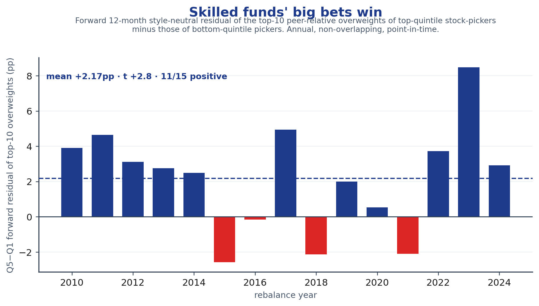
- Constituent-level verification. Audited directly at the holdings, the ten largest peer-relative overweights of top-residual managers outperform the bottom quintile's by +2.2pp forward (t ≈ 2.8), strengthening to +3.2pp (t ≈ 4.0) on the top five — a monotone conviction-to-residual relation that links the residual signal back to the securities managers actually chose.
- Allocator use. Inside a chosen mandate, rank candidate funds on their stock-selection residual, favor the top quintile, and hold — a gross ranking signal that improves forward odds, not a guarantee about any single fund. The signal is gross and holdings-derived; whether it survives net of fees is a separate question, and this is not a claim that active management broadly beats indexing net of fees.
A separate question — which residual best ranks managers on that skill — is addressed in Section 5; its t-statistics are not the persistence headline and are not interchangeable with the +2.3pp / t ≈ 3.4 result above.
1. What a fund's own documents reveal
Take two of the largest, most storied active US equity funds. Their public materials state what they aim to do in a single sentence each:
- Fidelity Contrafund (FCNTX, ~$146B): "The investment seeks capital appreciation." The strategy adds that it "invests in securities of companies whose value the advisor believes is not fully recognized by the public … in either 'growth' stocks or 'value' stocks or both," selected by "fundamental analysis."
- American Funds The Growth Fund of America (AGTHX): "The fund's investment objective is to provide you with growth of capital," pursued through a "flexible" mix of "traditional growth stocks as well as cyclical companies and turnarounds."
Both descriptions are accurate, and both are statutory mandates with no cross-sectional explanatory power: "seek capital appreciation through fundamental analysis of growth or value stocks" could be printed on the cover of almost any active equity fund, so it cannot identify an ex-ante idiosyncratic edge in any one of them. The disclosure is a qualitative label, not an estimable parameter.
The numbers the fund companies publish reduce to just two things, and neither isolates skill:
| What the materials disclose | What it actually tells you |
|---|---|
| Total return (shown against the S&P 500) | How much the fund made. A high number could be market, style, sector, luck, or genuine selection — the document cannot say which. |
| A market beta — sometimes, and loosely defined | AGTHX's own page lists a beta of 1.18 vs the S&P 500 over a trailing 3 years. But the S&P 500 is not its style benchmark, the window is arbitrary, and one beta collapses every kind of exposure into a single number. Contrafund's fact sheet shows no beta at all — only a 1-to-5 "risk level" dial and a category-relative Morningstar risk label. |
And the single coefficient it does provide is unstable. A returns-based market beta is an OLS estimate over a chosen look-back window; computed from public NAV returns, AGTHX's β to the S&P 500 is 1.20 over a trailing 3 years (reproducing the 1.18 the page reports) — but the estimate is strongly window-dependent, ranging across roughly a third of its own magnitude over rolling 3-year windows since 2006:
| Trailing window | AGTHX beta vs S&P 500 | FCNTX beta vs S&P 500 |
|---|---|---|
| 1 year | 1.21 | 0.92 |
| 3 years | 1.20 | 1.02 |
| 5 years | 1.13 | 1.03 |
| 10 years | 1.07 | 1.02 |
| rolling-3yr range, 2006–26 | 0.90 – 1.20 | 0.82 – 1.11 |
So β = 1.18 is not a structural property of the fund; it is one estimator's output for one window, and the window choice moves it by ~0.3 — severe parameter instability in a quantity meant to summarize risk (AGTHX at least labels its window; Contrafund's fact sheet reports no beta and no window at all).
The latent-factor confound
The window-dependence above is not sampling noise; it is a structural symptom of model misspecification. A single returns-based market beta is forced to serve as a catch-all proxy for a time-varying matrix of underlying factor exposures, and because the regression omits explicit controls for sector structure, subsector tilts, and style premia, the estimator suffers from omitted-variable bias on two margins:
- Factor leakage into the slope. When a fund is tilted toward a high-beta sector (technology) or a style block (small-cap growth), the OLS estimator mechanically compresses those distinct exposures into β_mkt. The coefficient stops measuring broad-market sensitivity and becomes a blend of unmodeled sector and style covariances — which is precisely why it wanders as those cross-sectional correlations shift over time.
- Windfall absorption by the intercept. Symmetrically, when an omitted layer enjoys a cyclical tailwind, the single-factor model misattributes that systematic return to the intercept, α. What returns-based scorekeepers report as "manager alpha" is frequently unmodeled, replicable, systematic risk riding along in the model's blind spot.
Both failures share a root cause: portfolios are dynamic — managers continuously adjust selection, sector concentration, and subsector exposure — while a returns-based beta imposes a static, average linear relationship over a 36- or 60-month window. A static estimator cannot track point-in-time exposure shifts; it lags, destabilizes, and fails out of sample. To isolate stock selection directly, this paper therefore uses a holdings-based decomposition rather than a returns-based regression — the cascade of Section 2, in which each layer is measured bottom-up, position by position, point-in-time as an accounting identity on the portfolio, rather than recovered as a window-dependent regression coefficient.
So from the offering materials an allocator can see, at best, how much the fund returned and roughly how much it moves with the market — and even that market sensitivity is poorly anchored. What they cannot see is the thing they are actually buying: did the return come from style, from sector bets, or from picking individual stocks?
2. What their holdings reveal
There is far more information available — it just isn't in the marketing. Every US mutual fund reports its full portfolio holdings every quarter to the SEC. The fact sheets even print a snapshot: Contrafund's latest filing shows 25.8% technology and 22.2% communication services, with a top ten running Meta, NVIDIA, Amazon, Berkshire Hathaway, and Alphabet. But that is a single static picture of what they hold today — not how those positions performed, and not why.
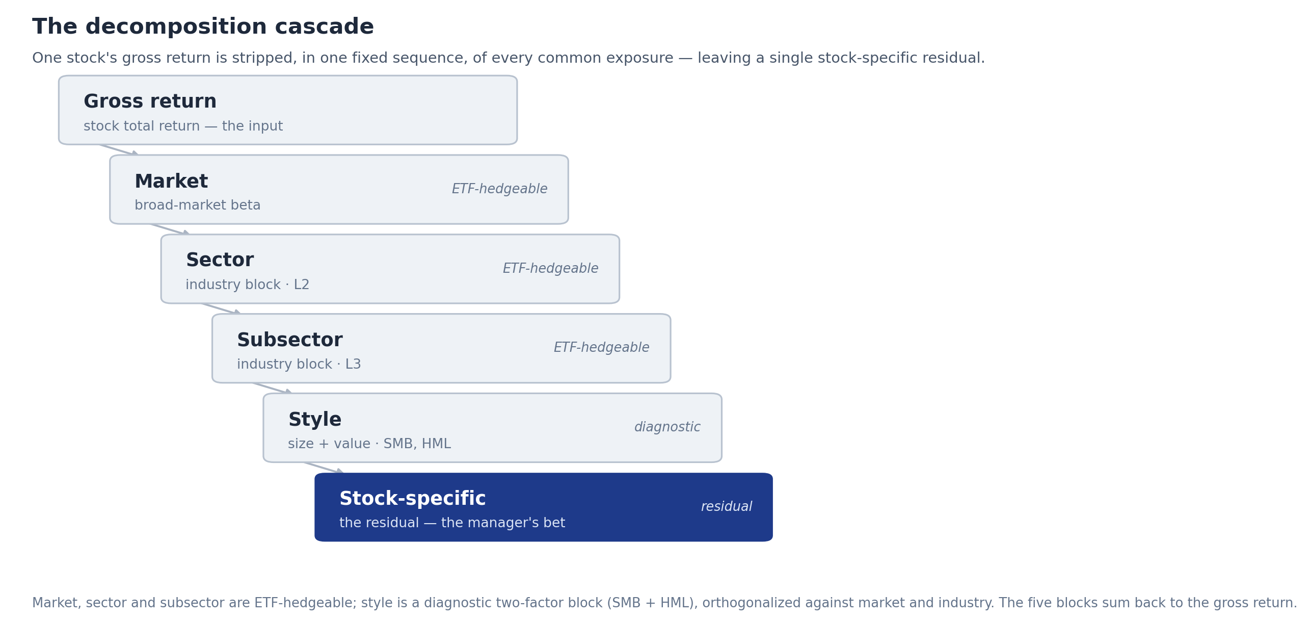
The RiskModels Holdings-Based Return Decomposition turns the full history of those quarterly positions into the answer. It is bottom-up: because we know what each fund held at each point in time, and we have already decomposed every underlying stock's daily return into its market, sector, subsector, and style layers, we can rebuild each fund's realized return stock by stock and split it into the pieces the fund documents cannot:
- how much came from simply being in the market,
- how much from style — a persistent size or value lean,
- how much from sector and subsector tilts,
- and how much from picking individual stocks — the residual left once the first three are stripped away.
The decomposition is a single sequence — market, then sector and subsector (the industry cascade), then a final size/value block (the Fama–French "ff2" strip) on top — and what remains after the full sequence is the residual used in this test — the component most directly associated with stock selection. The rest of this paper puts it to the test.
Why holdings-based and point-in-time matters. Unlike returns-based factor regressions, this design is holdings-based and point-in-time at both the fund and the position level. It therefore asks a different question: not whether a fund's historical return intercept persists, but whether the stock-specific return generated by the stocks it actually held persists once common exposures are removed. The distinction is what makes the test time-safe — every residual in any month is built only from positions an investor could have known then, decomposed with factor estimates that use no future data — and it is why the result speaks to identifiable, ex-ante selection rather than a byproduct of an end-of-sample regression fit.
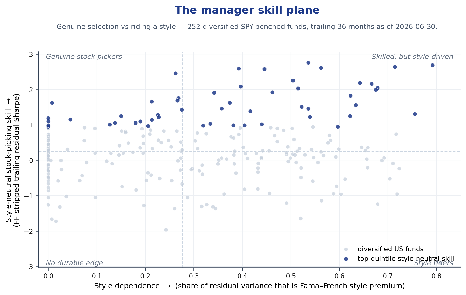
One picture frames where this leads. Place every diversified US equity fund on two axes: how much of its residual is just style premium (horizontal), and how much style-neutral stock-picking is left once that premium is stripped (vertical). The managers an allocator actually wants live in the upper-left — real selection, little reliance on a style tilt. The lower-right is where a value or growth bet is doing the work that looks like skill. The remaining question is whether this vertical axis predicts forward outcomes — and whether it is the only axis that does.
How this differs from the conventional tools
The established tools stop short of isolating stock selection:
| Tool | What it gives you | Isolates stock-picking? |
|---|---|---|
| Holdings look-through / "X-Ray" (Morningstar) | current sector / style-box / region weights | No — exposures, not return, not skill |
| Brinson attribution | active return → sector allocation + within-sector selection | Partial — "selection" still contains style/size bets (no factor control) |
| Morningstar Direct Global Risk Model | factor exposures + a security "specific return" (8 style + 11 sectors, 5-yr rolling regression) | Closer — but a flat factor model: 11 sectors, no subsector, noisy multi-year betas |
| This work | return → market / style / sector / subsector / stock-specific, then persistence-tested | Yes — bottom-up, one level deeper (to subsector), and validated which part is selectable skill |
Two differences matter. First, ours is bottom-up and goes one level deeper — to subsector: it removes the actual market, sector, and subsector (one level below the industry's 11 sectors) peer-group return directly, then strips Fama–French size/value — rather than regressing each stock on a fixed set of broad factors. Second, and more important, it adds the step none of these tools provide: it tests, out of sample, which decomposed components actually persist — and (as the rest of this paper shows) only stock-picking does. A risk model reports what happened; it does not tell an allocator that the selection piece is the only one worth selecting on.
Related to Active Share, but different. This work is related to Active Share — the widely used measure of how much a manager's holdings differ from its benchmark — but it asks a different question. Active Share asks how different a manager is from a benchmark; this paper asks which part of that difference actually persists: style, sector, or stock selection. Active difference is necessary for active skill to matter, but it is not evidence of skill by itself — and only one component of that difference (stock selection) persists here. (Active Share is taken up directly in a companion paper.)
3. The point-in-time testing framework
The empirical problem is one of identification before estimation: precisely which component of active return is being tested, and whether that component is observable point-in-time from holdings. Everything that follows runs inside one fixed framework — and the framework is the point. At each year-end we form the fund universe as it existed then (point-in-time membership, no survivorship hindsight), read each fund's positions as of their report date (the period the holdings describe), carry them forward, and decompose them into the cascade above using factor estimates that see no future data — then score a trailing-skill sort against a strictly forward, non-overlapping outcome window, so no observation is reused and the returns side carries no look-ahead. One timing assumption remains explicit and is tested separately: report-date holdings become public only when the fund files, up to ~60 days later, so the trailing feature's most recent quarter is not yet actionable in real time; §5 re-runs the test on ~60-day-stale (filing-lagged) holdings and the signal survives. The stock-selection residual is the target; style timing and sector timing, run through the identical machinery, are negative-control signals.
An allocator has already chosen a mandate ("I want a large-cap US stock fund") and now must pick which fund. They want evidence of a repeatable stock-selection component, not a return record driven by luck or by transient exposure. So we ask, of everything a manager actually does, which parts repeat — because only the parts that repeat are worth selecting on. For each layer of the decomposition above, the test is a single, plain question: if a manager was good at it over the past 3 years, are they still good at it over the next year?
How to read the score. Each year we rank funds into five buckets by their past skill at one thing, then watch what the top bucket does versus the bottom bucket over the next year, repeated across roughly fifteen years. The "reliability score" — a t-statistic of that gap across years — summarizes how dependable the gap was. We report simple annual, non-overlapping t-statistics to avoid overstating significance. Exactly one of three things happens:
| Score | What it means | What an allocator should do |
|---|---|---|
| +2 or higher | Persists — top stays top | Select on it |
| Between −2 and +2 | No pattern — mostly luck | Ignore it |
| −2 or lower | May reverse — directionally negative | Treat as a warning signal, not a standalone reversal trade |
A brief note on which statistic is the headline. Throughout, the persistence result is reported as a simple annual, non-overlapping t-statistic — chosen for legibility and because it does not overstate significance. (The fuller methodological history behind this choice, including statistics from an earlier framing that did not survive adversarial re-review, is documented in Appendix A.) The headline persistence number is the +2.3pp forward top-minus-bottom-quintile gap at t ≈ 3.4 reported in Section 4. A separate and distinct question — which residual best ranks managers on the stock-picking skill — appears in Section 5 and carries its own, larger t-statistics; those are not the persistence headline and the two should never be conflated.
4. What persists — and what does not
| Manager skill | In plain terms | Forward top−bottom gap | Score | Verdict |
|---|---|---|---|---|
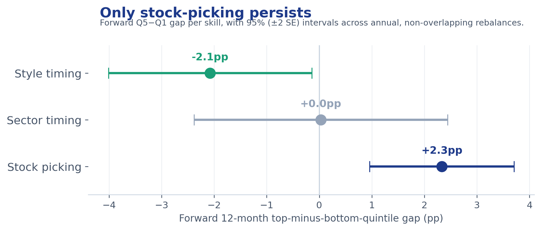
| Style timing | Leaning into value/small at the right time | −2.1pp | −2.1 | Weak/negative — recent style-timing success does not carry forward and is, if anything, a slight negative signal (not statistically reliable) |
| Sector timing | Overweighting the right sectors at the right time | +0.0pp | +0.0 | No pattern — sector bets don't repeat (held up even among the biggest sector-bettors) |
| Stock picking | Picking individual winners within sector & style | +2.3pp | +3.4 | Persists — the only component with reliable out-of-sample persistence in this sample |
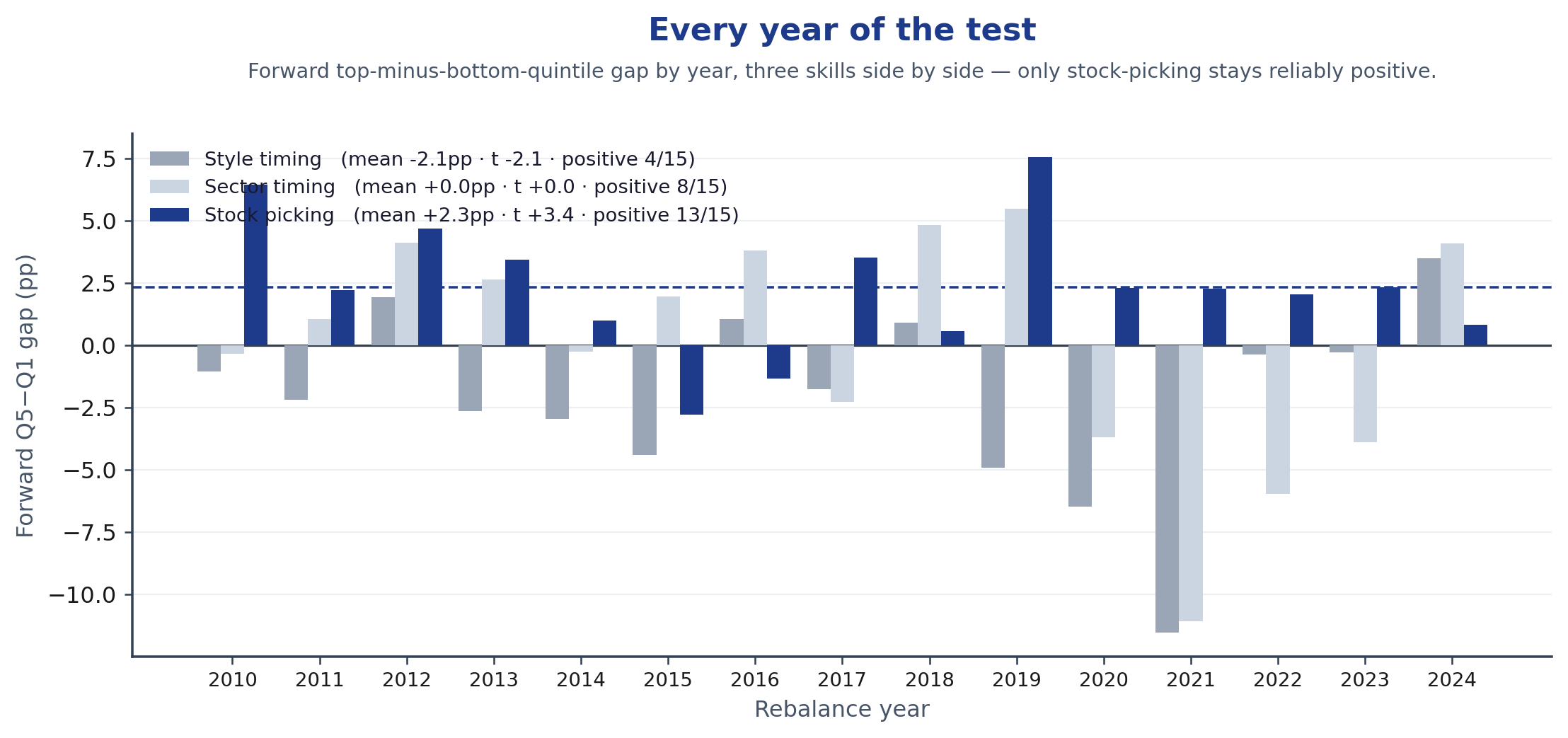
The stock-selection residual carries forward — a forward top-minus-bottom-quintile gap of +2.3pp with annual, non-overlapping reliability of t ≈ 3.4. Run through the identical machinery as negative-control signals, the other two components do not: recent style-timing success is a weak, directionally negative forward signal (t ≈ −2.1, not significant at the 5% level two-sided in this sample), and sector timing is indistinguishable from noise. Measuring all three the same way is the point — it is what rules out that the stock-selection result is a generic consequence of the validation machinery rather than a property of the residual.
How reliable is "t ≈ 3.4"? A transparency exhibit. Because the test is annual and non-overlapping, the whole result rests on roughly fifteen rebalances — a small sample by design, and we show every year of it rather than only the summary. The figure below plots the year-by-year top-minus-bottom-quintile gap for all three skills, with each skill's mean and a ±2 SE band. The pattern is consistent rather than driven by one or two extreme years: stock-picking is positive in 13 of 15 years (mean +2.3pp), style timing is positive in only 4 of 15 (mean −2.1pp), and sector timing is positive in 8 of 15 (mean +0.0pp) — a coin flip. The result holds in both halves of the sample (pre-2015 gap +2.5pp on six rebalances; post-2015 +2.2pp, t ≈ 2.7), and the cross-sectional Fama–MacBeth slope is reliable throughout (t ≈ 4.4). The early half rests on only six non-overlapping rebalances, so its standalone t is the noisiest cut in the paper; the deep pre-2019 N-Q history recovered for this revision lets those early years be measured against a materially broader set of funds, and the gap stays positive in both halves and survives a 16% widening of the cohort (Appendix A.1).
Effective sample size and multiple testing. Two cautions belong with any t-statistic built on ~15 annual observations. First, the trailing ranking feature is persistent (one-year rank autocorrelation ≈ 0.79) — which is the persistence we are documenting, not a defect. The statistic itself is built on the non-overlapping annual Q5−Q1 gap series, whose own year-to-year autocorrelation is ≈0 (+0.12), so the simple annual t uses the appropriate denominator. A stationary block-bootstrap on those gaps (respecting their mild dependence) gives P(mean ≤ 0) < 0.001. We retain humility about the modest 15-rebalance sample, but the feature autocorrelation does not deflate this t. Second, the design tests three skills plus a ranking bake-off; this multiple-comparison context was conceptually pre-specified (the three skills are the exhaustive decomposition of what a manager does, not a search over many candidate signals), but it is worth stating plainly — and the stock-picking result survives it: its raw two-sided p ≈ 0.004 becomes p ≈ 0.013 under Bonferroni, Holm, and Benjamini–Hochberg correction across the three skills, still significant at the 5% level. The robustness comes less from the nominal t than from the shape of the result: one skill reliably positive, one reliably negative, one flat, consistent year over year, and — as the next paragraph shows — concentrated in a between-fund level effect.
Between or within — where the persistence lives. How stock-picking persists matters for what an allocator should do with it. Split each fund's trailing-skill series into two orthogonal parts — the fund's full-sample mean (its long-run level, one number per fund) and each year's deviation from that mean (its timing) — and regress the forward outcome on both. Because the parts are orthogonal, the feature's forward predictive power (its R²) partitions exactly between them:
| Component of the trailing feature | Share of its variance | Share of its forward predictive power |
|---|---|---|
| Between-fund (long-run level) | 29.1% | 93.9% |
| Within-fund (year-to-year timing) | 70.9% | 6.1% |
Annual non-overlapping; 252 funds with complete trailing-and-forward data for this decomposition (of the 256-fund cohort), 3,098 fund-years; total predictive R² ≈ 6.0%. The two components are orthogonal, so the R² partitions exactly (Appendix A.5).
Most of the feature's variation is within-fund — 70.9% of its variance, as a fund's skill varies around its own average from year to year — but that variation is mostly transient noise. Of the feature's actual forecasting power, 93.9% is the between-fund level and about 6% is within-fund timing. A fund's durable average skill is what forecasts; its hot and cold years barely do. In plain terms, good stock-pickers stay good: the actionable form is identify the persistently good and hold, not chase whoever is hot this quarter. It is also why a ~15-rebalance sample suffices — a stable level is far easier to pin down than a flickering timing signal.
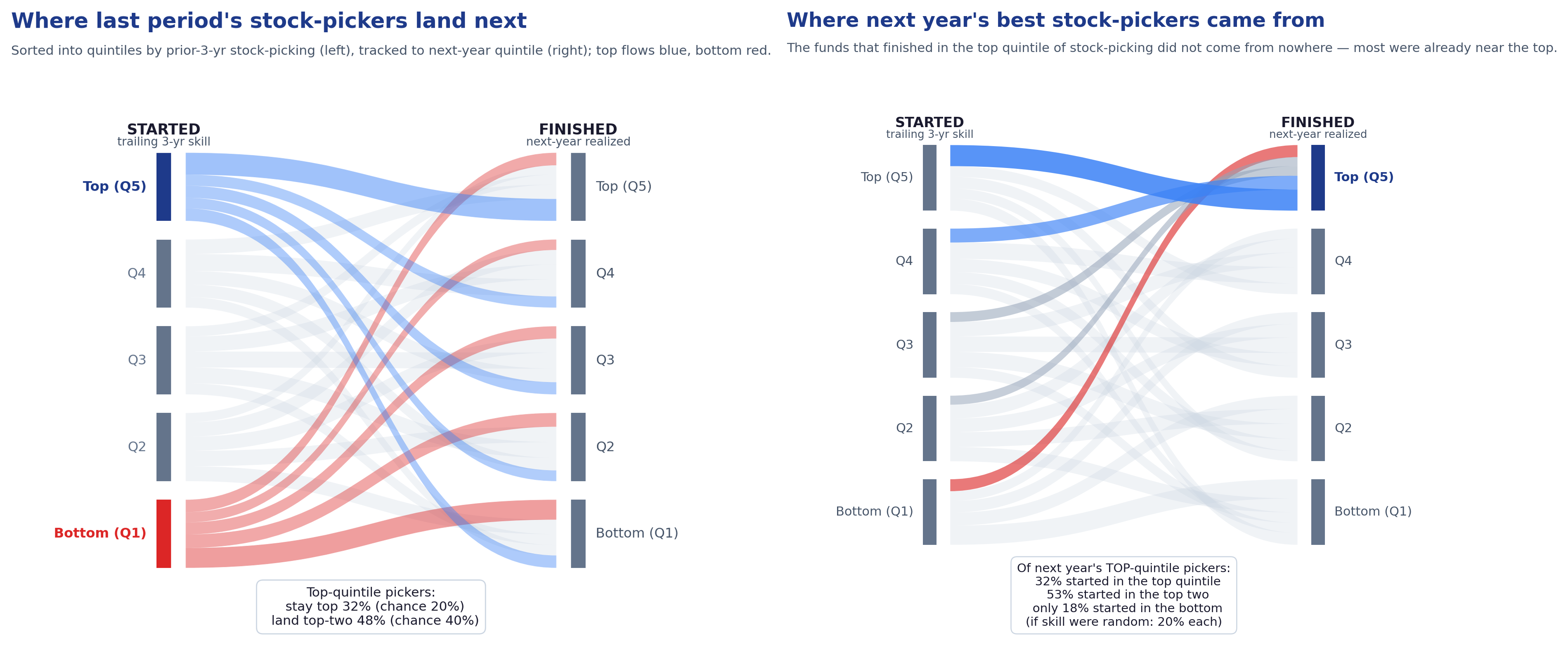
The same evidence reads both forward and backward. Read forward: where do this year's top stock-pickers land next year? Read backward — what an allocator actually faces — the managers who finished among next year's best, where did they start? Almost all were already near the top: of the funds that landed in next year's top stock-picking quintile, 32% started in the top quintile, 50% in the top two, and few in the bottom (against 20% each if skill were random). The strong group is drawn overwhelmingly from the previously strong group — which is exactly why ranking on trailing stock-picking and favoring the top tier improves forward odds.
Recent style-timing success is a weak, directionally negative forward signal, and it isn't a factor-reversal artifact. Funds that recently profited from a style lean tend to give it back — directionally negative and close to conventional significance (t ≈ −2.1), but not robust enough to treat as a standalone reversal signal. We checked whether this is just the style factors themselves mean-reverting year to year — it is not: the style factors do not meaningfully mean-revert at the annual horizon, and the negative signal lives in the timing component, not in a static value/growth tilt. A persistent style lean neither helps nor hurts selection; recent style-timing success is specifically a weak negative signal. The allocator conclusion is the same either way: do not credit a manager for recent style timing.
Sector timing is not distinguishable from noise in this sample (t ≈ 0). Sector/subsector timing shows no persistence in the full cohort. One natural worry is that closet-indexers dilute the measure — funds that barely tilt add noise. We re-ran the test among the funds that actually make the biggest sector bets (sorting directly on the size of their sector-timing contribution). It did not firm up; if anything it drifted slightly negative and stayed insignificant. Both timing skills fail to persist even among the funds that most actively do them, strengthening the interpretation that these components lack robust forward selection value in this cohort. (An earlier active-share filter appeared to lift sector timing toward significance, but that turned out to be a confound: active-share-versus-SPY flags funds that differ from the index at the stock level — i.e., good stock-pickers — so stock-picking skill was leaking into the imperfect sector-timing measure. The direct sector-bet-size filter removes the confound.)
5. Ranking managers on the one skill that persists
Section 4 established what persists. This section answers a different and narrower question: given that stock-picking is the skill worth selecting on, which residual best ranks managers on it? The statistics here measure the predictive power of a ranking feature against a fixed skill target — they are not the §4 persistence headline (+2.3pp / t ≈ 3.4) and are not interchangeable with it. A ranking-feature t can be larger than the persistence t because it asks an easier question (rank-order managers) on a different construct (feature-vs-target predictiveness rather than a forward portfolio gap).
The decomposition is sequential, not a menu of competing alternatives: each stock's return is stripped market → sector → subsector, and then a final Fama–French size/value block — "ff2" — is removed on top. (Earlier drafts framed the size/value strip as a separate, parallel "Fama–French cascade" competing with the sector cascade; in the current architecture it is simply the last block of one sequence.) The skill target is unambiguous: the residual after the full sequence, ff2 included — the style-and-sector-neutral residual. The one open choice is where in the sequence to read the ranking feature: at the raw sector-cascade residual (after subsector, before the ff2 block), or at the fully style-stripped residual (after ff2 as well). We score both against the same style-neutral target.
| Read the ranking feature… | In plain terms | Ranking t | Verdict |
|---|---|---|---|
| Before the ff2 block (raw sector-cascade residual) | market / sector / subsector stripped; size/value left in | 3.1 | For the fixed residual the two reads are roughly a wash; the decisive "read before ff2" edge is the adaptive residual (below) |
| After the ff2 block (fully style-stripped residual) | market / sector / subsector and size/value stripped | 3.5 | Comparable — stripping ff2 from the feature adds rolling-beta noise, but trailing style is non-persistent, so little net difference |
(The "ranking t" column measures how well each feature ranks managers on the style-neutral skill target — a §5 ranking question, distinct from the §4 persistence gap.)
A measurement lesson worth stating plainly. What you strip from the target and what you strip from the ranking feature are different decisions. The right target is style-neutral — the style-neutral residual is what is left once the ff2 size/value premium is removed. But the where-to-read choice bites hardest on the adaptive (L-Star) residual: read before the ff2 block it is the sharpest feature in the sweep (t ≈ 5.0) versus t ≈ 3.4 once style is stripped from it — stripping ff2 from the trailing feature injects rolling-beta estimation noise, and trailing style is non-persistent anyway, so leaving it in is harmless. (For the simpler fixed sector-cascade residual the two reads are roughly a wash, 3.1 vs 3.5.) Best practice is therefore an adaptive residual feature read before ff2, predicting a style-neutral target (read after ff2), and it is the basis for the screens in Section 7. In one line each:
| Role | Where it is read in the sequence |
|---|---|
| Feature (what you rank on) | Raw sector-cascade residual — before the ff2 block (market / sector / subsector stripped; size/value left in) |
| Target (what you score against) | Style-and-sector-neutral residual — after the ff2 block (market / sector / subsector and size/value stripped) |
A sharper ranking feature: the adaptive-hedge residual
The sector-cascade residual above hedges every stock all the way down to its subsector. A natural refinement is to let each stock choose how deeply to hedge — market only, market-plus-sector, or the full market-plus-sector-plus-subsector — picking the depth that best removes systematic risk for that stock rather than forcing the deepest level everywhere. L-Star — a point-in-time, cost-aware selection layer — chooses each stock's hedge depth to maximize predicted out-of-sample risk reduction net of hedging cost. An adaptive residual variant lets each stock choose its hedge depth point-in-time; in this sample it sharpens the ranking feature when read before the style strip, while still predicting the style-neutral target — a refinement to the ranking feature, not the headline persistence result.
Three residual variants appear below; each is one line:
| Residual variant | What it is |
|---|---|
| Raw residual | Return left after stripping market only — style and sector premia still inside |
| Full-depth (subsector) residual | Return left after hedging every stock all the way to subsector (the fixed sector cascade) |
| Adaptive (L-Star) residual | Return left after each stock hedges to its own cost-optimal depth (market, +sector, or +subsector) |
As a ranking residual the adaptive variant behaves in a revealing way. On the full 2006–2024 history (annual non-overlapping rebalances), the forward top-minus-bottom-quintile gap is below — each fund's per-stock L-Star residual is aggregated through its point-in-time holdings (a construction validated against the pipeline's own fixed-L3 residual at correlation ≈0.96). The columns vary how much style is then stripped from the feature — "before style-stripping," with style removed, and with style and momentum removed:
| Residual | before style-stripping | style-stripped | style + momentum stripped |
|---|---|---|---|
| Fixed full-depth (subsector) | +2.4pp (t ≈ 3.1) | +2.2pp (t ≈ 3.5) | +2.5pp (t ≈ 4.2) |
| Adaptive depth (L-Star) | +2.8pp (t ≈ 5.0) | +2.2pp (t ≈ 3.4) | +2.6pp (t ≈ 4.9) |
The adaptive residual is the sharper ranking read before style is stripped from the feature — +2.8pp / t ≈ 5.0 versus the fixed residual's +2.4pp / t ≈ 3.1 — and is the single most reliable feature in the sweep. Once style is stripped from the feature, the fixed and adaptive residuals converge (≈ +2.2pp, t ≈ 3.4–3.5): the adaptive edge is specifically a read-before-the-style-strip gain, which is exactly the best-practice configuration of this section (rank on the residual read before ff2, against a style-neutral target). (With momentum also stripped both sit near +2.5–2.6pp, t ≈ 4.2–4.9 — the adaptive advantage is a reliability-and-style-neutralization gain, not an unconditional one.) We verified out of sample that this extra edge is real stock-picking and not sector-timing riding along: purging the forward return of contemporaneous sector and subsector timing leaves the adaptive residual's advantage essentially intact, and a predictive test finds no channel by which the trailing signal could be forecasting future sector timing (Appendix A.9).
(These figures rank on a trailing residual feature against the same style-neutral target as §4, on the full 2006–2024 history; they are a §5 ranking comparison — they establish the relative sharpening from adaptive hedging, not a new headline number, and the effective-sample caveat of Section 4 applies.)
Seeing it in time: the cost of the filing lag
Everything above ranks funds on holdings as of their report date — the period the positions describe. But an allocator cannot act on a quarter's holdings until the fund actually files them, which for N-PORT is up to ~60 days after quarter-end. So the practical question is: how much of the ranking signal survives being acted on late?
The targeted correction: lag the feature. The look-ahead is confined to the most recent quarter — the only months in the 36-month trailing feature whose holdings are not yet filed at the rebalance date; the other ~33 months were filed long ago. So the surgical fix is to lag the ranking feature itself by ~60 days, dropping that one unfiled quarter from the average. On the §4 headline construction this barely moves anything: the forward Q5−Q1 gap changes by about 0.2pp and the reliability is unchanged — if anything slightly higher (t ≈ 3.3 → 3.5). An investor who ranked funds using only the holdings they had actually filed by the rebalance date would have selected essentially the same managers. A second, more aggressive check stales all holdings by 60 days and re-aggregates stock-by-stock through the same point-in-time positions, on the full history:
| Holdings basis (2006–2024, n = 18) | Forward Q5−Q1 | Reliability |
|---|---|---|
| Report date (as the positions describe the period) | +2.6pp | t ≈ 4.6 |
| ~60 days stale (the holdings an allocator could actually act on) | +2.8pp | t ≈ 4.8 |
Under this 60-day holdings lag the ranking is essentially unchanged — the trailing-skill feature is slow-moving, so modest staleness barely perturbs it. As a first pass this says the signal is durable enough to act on from public filings.
This is a robustness proxy, not the final word — and we flag its limits plainly. The proxy holds each fund's forward 12-month window fixed at a common anchor and only stales the holdings by a fixed 60 days. A faithful treatment is more involved on two fronts, both deferred to a follow-up (tracked in the backlog): (i) it must use the real per-filing availability dates (the N-Q reingest captures filing dates but has not yet propagated them to the returns panel), and (ii) because each filing becomes actionable at a different time, the forward 12-month windows shift per fund and per filing rather than sharing a common anchor. N-PORT's true availability is also quarterly plus ~60 days, so between filings the actionable holdings can be 2–5 months stale; a short real-availability sample (N-PORT era, 2019+) hints the fuller lag erodes the spread materially more than this gentle proxy. We therefore present this only as preliminary evidence of robustness to a modest lag, not as a sized cost-of-delay.
Bottom line. Of the three things managers do, recent style-timing success is a weak, directionally negative forward signal (not statistically reliable), sector timing is not distinguishable from noise in this sample, and only stock picking persists — as durable quality, not timing. The cleanest way to rank managers on that stock-picking skill is the raw sector-cascade residual read before the ff2 block (size/value left in the feature, stripped only from the target), and an adaptive, cost-aware version of it (L-Star) sharpens the ranking feature further when read before the style strip.
6. How the industry evaluates managers
Everyone in institutional manager selection is trying to answer the same question we are — which managers have repeatable stock-selection skill? The field splits into three camps, and the one thing almost no one does is the thing this work is built on: isolate stock-picking from style and sector bets, and publish evidence that the isolated signal predicts the future.
Allocator diligence commonly relies on style classification, sector allocation, benchmark-relative attribution, and recent performance patterns to evaluate active managers. Those measures are useful for describing what a fund owned and how it differed from its benchmark, but they are often poor evidence of repeatable skill. The critique is not that allocators ignore stock selection — it is that the standard toolkit detects difference without identifying which part of that difference repeats: it blends stock selection with style, sector, and subsector exposure, then asks the allocator to infer skill from a blended return record. In this sample, recent style-timing success is weakly negative out of sample, sector timing is indistinguishable from noise, and only the stock-selection residual persists — which reframes the allocator's question from "did this fund beat its benchmark?" to "did this fund generate repeatable stock-specific residual return after removing the replicable market, style, sector, and subsector exposures?"
| Provider | How they evaluate skill | Holdings-based? | Isolates stock-picking from style/sector? | Best published forward stat |
|---|---|---|---|---|
| Qualitative rating shops | ||||
| Mercer | Committee ratings A/B/C on people & process | No | No | No public forward statistic in materials reviewed (proprietary) |
| Aon | Buy/Qualified/Sell + ops + ESG; factor analysis internally | Internally | Internally, not published | No public forward statistic in materials reviewed |
| Wilshire | Qualitative scoring model | No | No | No public forward statistic in materials reviewed |
| Russell | Four P's (People/Process/Philosophy/Performance) + ML screen | No | No | Firm-reported high hit-rate for hire-rated products — blends asset classes, self-reported |
| NEPC | Conviction ratings | No | No | Median large-cap mgr earns less than its fee (active doesn't clear costs) |
| Returns-based scorekeepers | ||||
| Callan | % of rolling periods with positive net excess | No (rejects holdings) | No | Treats Active Share as risk, "not a litmus test" for skill |
| SPIVA (S&P DJI) | Survivorship-free persistence & win-rates on raw return | No | No (single-benchmark, total return) | Top-quartile persistence collapses toward zero within a few years; a large majority of active US funds trail over 5–20 yrs |
| Holdings-based predictors | ||||
| Cambridge Associates | Qualitative + active-share / concentration research | Yes | Partly (active share, not factor-neutral) | Higher active share / concentration → higher subsequent relative return |
| Morningstar — Global Risk Model | 36-factor risk model (11 sectors), security "specific return" | Yes (factor) | Partly (flat factor model) | Validated for risk forecasting, not skill |
| Morningstar — "best predictor" (Rekenthaler / Cohen-Coval-Pastor) | "Company they keep" — overlap with funds that have strong records | Yes | Carhart 4-factor alpha (no sector) | ≈ +330 bps top-vs-bottom subsequent alpha (global equity funds, 2004–2018) |
| This work | Bottom-up return decomposition through full PIT holdings | Yes | Yes — market + sector + subsector + style stripped | +2.3pp forward Q5−Q1, annual t ≈ 3.4, persistence-validated |
Three things separate the camps. Qualitative rating shops (Mercer, Aon, Wilshire, Russell, NEPC) rate managers on organization, people, process, and philosophy — thoughtful frameworks, but largely proprietary, and almost none publishes a quantified track record showing its top-rated managers add alpha. The most candid public number from the group is NEPC's: the median large-cap manager does not earn back its own fee. Returns-based scorekeepers (SPIVA, Callan) measure persistence and win-rates on raw total return against a single benchmark; they are rigorous and survivorship-free, and they supply the industry's most-quoted facts — raw top-quartile persistence collapses toward zero within a few years, and most active US equity funds trail over long horizons — but by construction they cannot separate skill from style or sector tilts. Holdings-based predictors (Cambridge, Morningstar) come closest: Cambridge ties higher active share and concentration to higher subsequent relative return, and Morningstar's Rekenthaler "best predictor" — the Cohen-Coval-Pastor "company they keep" consensus — is a holdings-based, style-adjusted quality-of-holdings score with a published forward spread.
The deeper distinction, though, is about what each approach can isolate and validate:
- Returns-based persistence tests don't isolate stock selection. A fund's record blends market, style, sector, and selection; raw persistence tests cannot say which component repeats.
- Holdings look-through shows exposures, not validated persistence. X-Ray and risk models report current weights or factor loadings — what a fund is, not which part of its skill carries forward.
- This work tests decomposed components out of sample. We strip market, sector, subsector, and style by construction, then ask which decomposed component persists — and report that only stock-picking does.
Positioning relative to existing methods
The published holdings-based forward spreads (Cambridge, Morningstar) and our stock-selection result are broadly the same order of magnitude — reassuring, but not a controlled comparison: the studies differ in universe, period, signal construction, and alpha definition (Morningstar scores a fund by the track records of other funds holding the same stocks; Cambridge uses active share; ours is the manager's own realized style-neutral residual). The accurate statement is "same order of magnitude," not "validated against each other." Full study-by-study differences are in Appendix A.6.
We ran a sharper test of whether this is identifiable stock selection: do skilled funds' big bets actually win? At each rebalance we sort funds into skill quintiles on trailing stock-picking, take each fund's ten highest-conviction positions — its largest overweights versus the peer-cohort consensus holding — and track those positions' forward 12-month style-neutral residual return. The overweights of top-quintile pickers beat the overweights of bottom-quintile pickers by +2.2pp over the next year (t ≈ 2.8, positive in 11 of 15 years, out of sample, 2006–2026) — and the spread strengthens as the bets concentrate (+3.2pp, t ≈ 4.0 on the top five positions). The persistence is not a fund-level statistical artifact; it lives in the specific, high-conviction, peer-differentiated stocks that skilled managers emphasize. A fuller treatment — index-relative weights, a replicable "best ideas of skilled funds" portfolio, and transaction costs — is the subject of a companion paper.
(For completeness we also implemented the standard academic consensus measure — the Cohen-Coval-Pastor "company they keep" score — on the same cohort; on a homogeneous large-blend universe it cannot discriminate, because when nearly every fund holds the same mega-caps the consensus is near-identical across funds. That is a known property of consensus signals on homogeneous cohorts, not an artifact of our implementation; detail in Appendix A.6.)
The specific synthesis. Each building block of this method is established — holdings-based selection signals, factor neutralization, out-of-sample persistence validation.
We are not aware of a single incumbent product or published manager-selection framework that combines all of: a signal that is holdings-based, factor- and sector-neutral by construction, and validated out of sample on which decomposed component persists.
The existing methods each fall short on one leg of that combination. Cambridge uses active share (not factor-neutralized); Morningstar's best predictor is style-adjusted but not sector-decomposed, and its risk model stops at 11 sectors and is validated for risk, not skill. The distinctive contributions of this design are (1) published, significance-tested evidence of which component persists — the principal edge, not granularity; (2) full factor-and-sector neutralization down to subsector; and (3) transparency — a decomposition reproducible through the underlying holdings rather than a proprietary rating. The extra subsector depth, tested head-to-head against a Morningstar-like sector-only version, is a reliability refinement (it steadies the year-to-year ranking) rather than a step-change in the size of the edge (Appendix A.6); the emphasis is the persistence-validation and transparency, not the granularity.
7. Implications for allocators
The practical implication is narrow and usable. This paper does not argue that active management beats passive net of fees — it narrows the allocator's search problem: if you are already allocating within an active mandate, it is a better way to rank the managers in it. When you have fixed a mandate and are choosing among funds inside it:
- Do not select on recent style-driven returns. A fund that just had a great year because value (or growth, or small-cap) had a great year is, if anything, a slightly negative forward signal (t ≈ −2.1, not statistically reliable in this sample) — don't credit recent style timing.
- Do not select on recent sector bets. Sector timing is not distinguishable from noise in this sample (t ≈ 0), even for the managers who bet hardest on it.
- Do select on style-and-sector-neutral stock-picking, and treat it as durable quality. It is the one component that carries forward, and it carries forward as a level — good pickers stay good — so the right behavior is to identify them and hold, not to chase whoever is hot.
How an allocator uses this signal in practice
A concrete decision framework, for choosing among funds inside an already-chosen mandate:
- Hold the mandate fixed. The signal ranks managers within a comparable cohort (e.g., large-cap US blend). It is not a tool for deciding active-versus-passive or for crossing mandates.
- Score each candidate on its trailing style-and-sector-neutral stock-picking — its sector-cascade residual over a trailing multi-year window, point-in-time (Section 5; Appendix A.2).
- Favor the top quintile and avoid the bottom. The forward edge is concentrated at the top of the ranking; the bottom is where style- and sector-driven records cluster.
- Hold, don't chase. Because the skill is durable between-fund quality, the right cadence is slow — re-rank periodically and replace only on a sustained drop, not on a single soft year (year-over-year top-quintile retention is roughly 59%; Appendix A.7).
- Treat it as odds, not certainty. Top-quintile membership raises forward odds (top-quintile funds stay top-quintile 32% of the time versus 20% by chance); it does not guarantee any single fund will outperform. This is a cohort ranking signal.
Limitations & scope
We lean into the transparency of this work as a strength, which means stating its limits plainly:
- Gross, not net; and the Berk-Green caveat. The signal lives on the gross, holdings-derived side, where skill demonstrably survives. Whether that skill reaches the investor is a separate question: skilled managers may capture the rents themselves through fees or asset growth (Berk-Green). Nothing here claims most active managers beat their benchmark net of fees — the returns-based evidence that most do not is real.
- Cohort scope. The result is established on a diversified US large-cap equity cohort. We do not extend the headline to sector funds, international, small-cap-only, or non-equity mandates; the framework is portable, but the specific numbers are not.
- Survivorship and backfill. While the security-level cascade covers ~6,300 securities including delisted names, the fund cohort is drawn from funds extant at the panel's final date and back-filled through history — it does not include funds liquidated, merged, or renamed before the panel end, and so carries survivorship and backfill bias. We bound it with survivorship-hardened re-runs (fixed-survivor and balanced-panel subsamples), where the result holds or strengthens (t ≈ 3.3). The direction of this bias is not fully resolved without a survivorship-free dead-fund overlay. The survivor-hardened subsamples are reassuring, and the allocator use-case — ranking among extant candidate funds — is partly insulated, but the definitive test is to add liquidated, merged, and renamed funds in a future revision (Appendix A.1).
- Modest sample. The test rests on ~15 annual rebalances. The trailing feature is persistent (autocorrelation ≈0.79) — the very persistence being documented — but the t is built on the non-overlapping annual Q5−Q1 gap series, whose own autocorrelation is ≈0 (+0.12), so the simple annual t uses the appropriate denominator (Section 4; Appendix A.4, A.8).
- The adaptive-hedge refinement is a reliability gain, not a larger edge. The adaptive (L-Star) residual gives a more reliable ranking signal read before the style strip (Section 5; +2.8pp/t ≈ 5.0 vs the fixed residual's +2.4pp/t ≈ 3.1 on the full 2006–2024 history); once style is stripped from the feature the two converge (≈ +2.2pp, t ≈ 3.4–3.5). We present it as a refinement of the ranking residual, not as a replacement for the §4 persistence headline.
Final framing
What this work claims is narrow and, we think, useful: if you are going to select an active manager inside a chosen mandate, the decomposition tells you which part of their record is worth selecting on, and the answer — out of sample, on legible statistics — is stock-picking, measured style- and sector-neutral, and treated as durable quality. The underlying RiskModels decomposition lets allocators apply this framework to their own mandates and candidate lists.
Data & verification. Our own statistics are computed in-house on the cohort and panel described in Appendix A and are stated plainly. External comparisons are directional unless explicitly stated otherwise, because the cited studies differ in universe, period, signal construction, and return definition. Third-party figures cited in the comparison table were checked against the referenced source materials as of June 2026.
Appendix A. Methodology
A.1 Sample construction
Cohort definition (at each rebalance). The cohort is, at each rebalance, SPY-benchmarked (BW-BENCH-SPY) US equity funds with coverage-quality "high" or "medium." The intended universe is diversified US equity; after the SPY-benchmark and name filters the realized cohort is effectively entirely the large-cap-blend group (the panel's style_group field is a coverage-derived tag, not a prospectus label, so style breadth is enforced by fund-name filtering rather than a reliable style classifier). Sector, specialty, international, and passive products are excluded by name. The numbers therefore characterize a large-cap US-blend cohort specifically. This yields 256 funds total across the sample, 15 annual rebalances, with 100–251 funds per cross-section (median 202), over 2006–2026 — widened in v1.4 by 36 active funds whose pre-2019 N-Q history was recovered for this revision.
Effect of the widening on early-year dispersion. The 36 added funds are ~10% of the early (pre-2015) cross-sections and are individually less cross-sectionally dispersed than the incumbents (trailing-feature σ ≈ 0.021 vs 0.039). Their entry nonetheless reshuffled the quintile breakpoints and added idiosyncratic tail noise: the early-half Q5−Q1 mean rose modestly (+2.12 → +2.30pp) while its year-to-year volatility rose more (2.33 → 3.12pp), which is why the early-half t falls from ≈ 2.2 to ≈ 1.8 even as the mean improves. The persistence direction is unchanged in every comparable year; the widening trades a little mean for more variance in the thin early cross-sections, and we report the wider, more conservative cohort as the headline rather than the tighter 220-fund subsample.
Rebalance convention. Each rebalance is taken at each calendar year's last available observation — annual and strictly non-overlapping.
Feature and outcome windows. The ranking feature is the trailing-36-month mean of the relevant skill (minimum 24 monthly observations required); the outcome is the forward 12 months.
Decomposition engine. The underlying engine runs a bottom-up cascade on a security-level universe of ~6,300 distinct securities including delisted names across ~5,000 trading days, decomposing every stock, every day, through one sequence — market / sector / subsector layers (the "sector cascade") followed by a size/value block (the Fama–French "ff2" strip) on top. Stock residuals are aggregated to funds through their actual reported point-in-time holdings — SEC N-PORT for recent history and a restored N-Q deep history before 2019. The fund cohort, however, is drawn from funds that exist as of the panel's final date and is back-filled through history; it therefore does not include funds liquidated, merged, or renamed before the panel end, and is subject to survivorship and backfill bias. We bound this by re-running on survivorship-hardened subsamples — funds present from the panel start (first observation ≤ 2006) and the balanced panel present at every rebalance — where the gap holds at roughly +1.9 to +2.0pp and the t stays strong (≈ 2.7 on the early-start subsample, ≈ 3.5 on the balanced panel); the result also survives dropping the bottom quintile entirely, so it is not an artifact of truncating poor performers. A partial dead-fund overlay now exists: the intensive N-Q recovery behind this revision restored pre-2019 holdings for the deterministically recoverable liquidated/merged funds (the long-tail of renamed and odd-format dead funds, and delisted funds whose holdings are not yet ingested, are still deferred), so the pre-2019 sample is no longer survivor-only and the early-half persistence (Section 4) is measured against a materially larger set of funds that did not all survive. The direction of the residual bias falls mainly on the spread (a survivor-only sample likely understates the bottom quintile, biasing the gap downward if anything), not the level; the definitive test remains adding the full liquidated/merged/renamed universe — including the deferred long tail — in a future revision. Holdings are carried forward from their report date (the period they describe), so the returns side carries no look-ahead — a fund's residual in any month is built from the positions it actually held. The one residual timing assumption is availability: report-date holdings are not public until the fund files them, up to ~60 days later, so the trailing feature's most recent quarter is not yet actionable in real time. We do not paper over this — §5 re-runs the ranking on filing-lagged (~60-day-stale) holdings and the signal survives; a faithful per-filing availability treatment is tracked as follow-up (the N-Q reingest captured filing dates but has not yet propagated them to the returns panel). Holdings are treated as static between filings (a conservative carry-forward).
The broader panel from which the cohort is gated contains on the order of ~170,000 coverage-gated fund-months across ~1,000 funds; the manager-selection tests in Sections 4–5 run on the diversified SPY-benched cohort described above.
Subsector is the finer industry grouping one level below sector.
A.2 The decomposition
Each fund's return in month t is rebuilt as the holdings-weighted sum of its stocks' decomposed returns, using only positions known as of t (point-in-time):
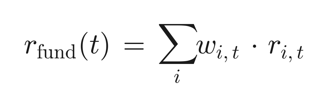
with the weights w_i,t taken from the latest filing on or before t.
Each stock's daily return is decomposed two ways. The two cascades produce two residuals:
-
Sector-cascade residual — the part of return orthogonal to industry structure:
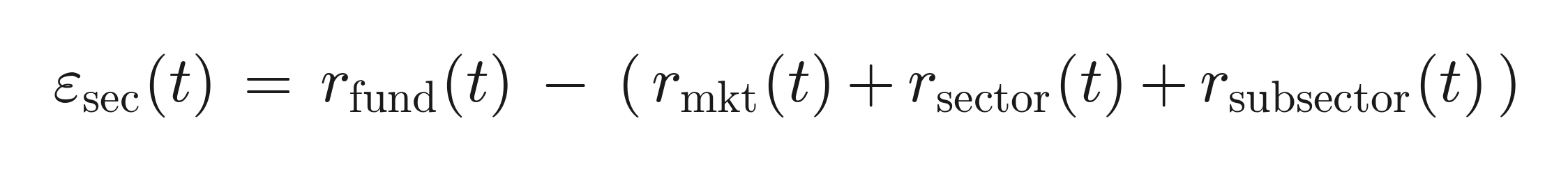
-
Fama–French-cascade residual — the part orthogonal to style:
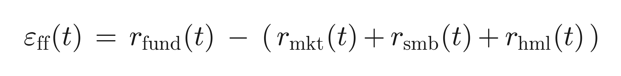
-
Doubly-cleaned stock-picking — the part orthogonal to both industry structure and style:

This residual, ε_pick(t), is the paper's structural parameter — the idiosyncratic, non-systematic component of performance whose out-of-sample, cross-sectional stability the rest of the paper tests. It is the stock-selection target throughout.
Point-in-time style neutralization. Style is stripped strictly point-in-time. For each fund and month t, the rolling factor betas are estimated by OLS on a strictly trailing 36-month window ending at t (no look-ahead):
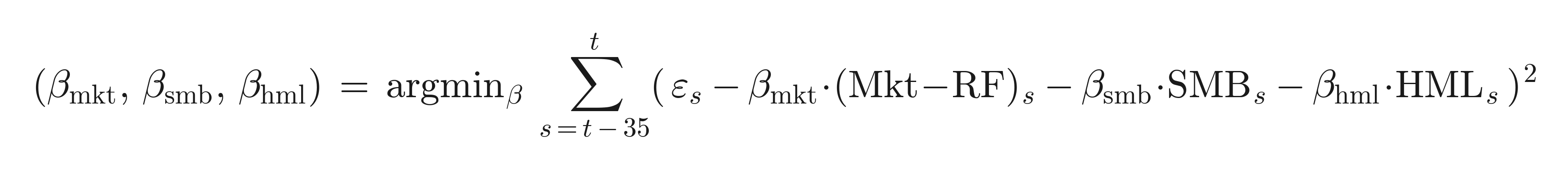
and the style-neutral residual is that residual minus its fitted style component:
Because the window ends at t, the neutralization uses only information available at the time.
Why an ff2 style block (size + value), not Carhart (with momentum). We use an ff2 style block — SMB and HML — rather than a broader Carhart-style block that includes momentum. The reason is conceptual and practical: the paper's target is persistent stock-selection skill read from holdings, not short-horizon price-continuation exposure. Momentum is therefore treated as a robustness dimension rather than part of the primary style definition. Section 5 repeats the ranking comparison after additionally stripping momentum; the stock-selection result does not depend on omitting it.
A.3 The three skill axes
The three manager skills tested in Section 4 are constructed from the cascade layers (the market/beta layer is excluded — it is not a selectable skill):
- Style timing = the fund's size/value contribution (β_smb·SMB + β_hml·HML) inside the residual. Section 4 further decomposes this into a static tilt (β̄·factor, using the fund's own mean exposure) and a timing component ((β_t − β̄)·factor); the anti-persistence lives in the timing component, with the static tilt neutral.
- Sector/subsector timing = the ERM3 sector and subsector layers (systematic return net of the market layer).
- Stock picking = the style-neutral residual (residual net of size/value).
A.4 The test: train → predict → roll-forward
Symmetric validation design. The design is symmetric across three candidate manager-selection signals — style timing, sector timing, and stock selection. For each, the identical estimator, windows, cohort, and forward horizon test the one-sided hypothesis that its trailing value carries no forward cross-sectional information (H₀: E[Q5−Q1 forward gap] ≤ 0). Only stock selection rejects H₀ out of sample; style timing and sector timing do not. Because the machinery is held fixed and only the target component changes, the differential survival supports the interpretation that the result is specific to the stock-selection residual — not a generic sorting effect, and not a specification selected to fit the data.
The headline design is an annual, non-overlapping train → predict → roll-forward. At each year-end, funds are ranked by their trailing-36-month skill at the relevant axis (point-in-time). The next 12 months' top-quintile-minus-bottom-quintile (Q5 − Q1) contribution in the relevant payoff space is recorded. This repeats across 15 annual rebalances. The reported "score" is the simple t-statistic — mean over standard error — of that annual gap series. We deliberately use this legible annual t rather than information-ratio or bootstrap statistics as the headline; the latter, when applied to overlapping monthly windows, inflate significance and do not annualize cleanly.
Effective sample size and multiple testing. The trailing ranking feature is persistent — its 1-year rank autocorrelation is ≈ 0.79 — which is the persistence we are documenting, not a defect. The statistic itself is built on the non-overlapping annual Q5−Q1 gap series, whose own year-to-year autocorrelation is ≈0 (+0.12), so the simple annual t uses the appropriate denominator. A stationary block-bootstrap on those gaps (respecting their mild dependence) gives P(mean ≤ 0) < 0.001. We retain humility about the modest 15-rebalance sample, but the feature autocorrelation does not deflate this t. On multiple testing: the design evaluates three skills (Section 4) plus a ranking bake-off (Section 5), a context worth stating, but these were conceptually pre-specified — the three skills are the exhaustive decomposition of what a manager does (style timing, sector timing, stock selection), not a search across many candidate signals. The stock-picking persistence survives this correction: raw two-sided p ≈ 0.004 → adjusted p ≈ 0.013 under Bonferroni, Holm, and Benjamini–Hochberg (m = 3), still significant at 5%.
A.5 Level vs timing (the fixed-effects test)
To separate durable quality from timing, decompose each fund's trailing stock-picking feature into a permanent fund-level mean and a year-to-year deviation:

where μ_i is the between-fund level (the fund's full-sample mean — one number per fund) and ν_{i,t} is the within-fund deviation (each year's departure from that mean). Because within-fund deviations sum to zero, the two components are orthogonal across the panel, so regressing the forward outcome on both jointly partitions the predictive variance exactly: R² = R²_between + R²_within, with each R²_k = β_k² · Var(component_k) / Var(y). On the annual non-overlapping panel (252 funds with complete data for the decomposition, of the 256-fund cohort; 3,098 fund-years) the total predictive R² is ≈ 6.0%, of which the between-fund level accounts for 5.6% and the within-fund deviation 0.4%. The level therefore carries 93.9% of the feature's forecasting power and timing about 6%. The persistence is a between-fund level effect: some funds are persistently better pickers, rather than any fund switching its picking on and off.
We report these variance shares rather than regression t-statistics by design. A cross-sectional regression across funds treats the 252 funds as independent observations, but funds alive in the same years share common annual shocks, so such a t overstates significance. The significance of the persistence is the annual non-overlapping t ≈ 3.4 of Section 4, which respects that the independent dimension is the ~15 years, not the cross-section. This is why the allocator prescription is "pick the persistently good and hold," not "time the hot hand."
A.6 Does the skill show up in the stocks? The conviction test (plus bake-off and CCP)
Conviction test (primary). The sharpest check that the fund-level persistence is identifiable stock-selection is whether skilled funds' large positions outperform unskilled funds' large positions. At each annual rebalance we rank cohort funds into skill quintiles on trailing stock-picking, take each fund's ten largest overweights versus the peer-cohort consensus holding, and compound those stocks' forward 12-month style-neutral (subsector) residual, strictly after the report date (point-in-time). The top-quintile minus bottom-quintile spread is +2.17pp / t ≈ 2.78, positive in 11 of 15 years on the 256-fund cohort, 2006–2026. It is monotone in conviction — +3.17pp / t ≈ 3.98 on the top five, +1.70pp on the top twenty — and stronger conviction-weighted than equal-weighted, the signature of a "best ideas" effect (Cohen-Polk-Silli) conditioned on skill. The index-relative variant (overweight versus actual SPY constituent weights) corroborates at +2.95pp / t ≈ 1.90 over the post-2019 window where SPY weights are available. This is the validation the §6 figure shows; a full treatment (reconstructed full-history index weights, deciles, a replicable portfolio, costs) is deferred to a companion paper.
Bake-off (subsector vs sector-only) [carried from the prior 220-panel; directionally unaffected by the widening]. Identical pipeline, annual non-overlap, both sides style-neutralizing the ranking signal to isolate the industry-depth question: sector-only +2.31pp (t ≈ 2.79) vs subsector +2.62pp (t ≈ 3.14). Subsector depth reduces noise and lifts reliability; it does not materially enlarge the edge — a refinement, not the headline.
CCP "company they keep" (carried). We also implemented Cohen-Coval-Pastor on the cohort (a fund's skill proxy is its trailing CAPM alpha; a stock's "quality" is the leave-one-out holdings-weighted average skill of its holders; a fund's score is the holdings-weighted average quality of its stocks). On a homogeneous large-blend cohort it scored ≈ noise (t ≈ 0.7) while our residual sorted — a structural property of consensus measures on homogeneous universes (when every fund holds the same mega-caps the consensus is near-identical across funds), not a claim that we beat it everywhere. The conviction test above supersedes this as our "is it real skill?" evidence.
A.7 Capacity
Year-over-year top-quintile retention is ~59% (turnover ~41%/yr → implied mean holding ≈ 2.4 years). For a manager-allocation signal this is highly tradeable — re-allocation roughly every 2.4 years sits well inside fund lock-up and redemption constraints — and the slow 36-month feature gives durable selection.
A second, distinct dimension of tradability sits one level down, at the holdings level: how slowly the underlying positions turn. The manager-ranking turnover above measures how often an allocator re-sorts funds; position retention measures how stable each fund's own portfolio is between filings. The signal is built on a trailing-36-month residual aggregated through point-in-time holdings that are themselves persistent, so the feature does not swing on quarter-to-quarter position churn. Slow underlying-holdings turnover reinforces the slow re-allocation cadence: both the ranking and the positions that generate it move gradually, which is what makes the signal practical to act on rather than a high-frequency trade.
A.8 Honest caveats
- The defensible significance is the annual, non-overlapping, simple-t statistic. The headline configuration (Section 4) — the symmetric style-neutral stock-picking test (a style-neutral feature against a style-neutral target) — is +2.3pp forward Q5−Q1 at t ≈ 3.4, and this is the single number used throughout the paper. For ranking managers, reading the adaptive (L-Star) residual before the ff2 size/value block (the best practice of Section 5) is sharper still (≈ +2.8pp, t ≈ 5.0) — but that is a Section 5 ranking statistic on an easier question, not the Section 4 persistence headline, and the two are not interchangeable. An earlier framing of this work used a Newey–West t on overlapping monthly windows together with a monthly information ratio; adversarial re-review showed those overstated the result — the "monthly" observations were overlapping twelve-month windows that do not annualize cleanly, and a large part of the apparent signal was a permanent level difference between funds rather than a timed bet. Those statistics are deliberately not used here; the conservative annual t is.
- Stock-picking persistence is a between-fund level effect, not a timing signal an allocator must catch in motion (A.5).
- The 1-year feature-rank autocorrelation is high (≈0.79) — which is the persistence we are documenting, not a defect — but the t is built on the non-overlapping annual Q5−Q1 gap series (own autocorrelation ≈0), so the simple annual t uses the appropriate denominator and the feature autocorrelation does not deflate it (full statement in A.4).
- Part of the negative style-timing signal reflects the tendency of a rolling exposure's deviation from its own mean to revert toward it; either way, the allocator conclusion (don't credit recent style timing) is unchanged.
- This signal lives on the gross / holdings-derived side, where skill demonstrably survives. The Berk-Green caveat stands: the rents to genuine skill may accrue to managers rather than investors.
- The adaptive-hedge (L-Star) residual is included (Section 5; construction and the out-of-sample leakage check in A.9). An earlier explained-ratio issue in cloned pre-launch ETF history (XLC, XLRE) has been resolved in the cascade; the L-Star results here run on the current, materialized cascade, whose PIT-safe, GBM-based selection algorithm is a point-in-time refinement to the ranking feature.
A.9 The adaptive-hedge residual (L-Star)
Construction. The fixed sector cascade hedges every stock to the deepest level (market → sector → subsector). The adaptive residual instead lets a cost-aware, PIT-safe, GBM-based selection algorithm choose each stock's hedge depth (market, market+sector, or market+sector+subsector) to maximize predicted out-of-sample risk reduction net of hedging cost, rather than always hedging to the deepest level. It is computed point-in-time — a refinement to the ranking feature, not the headline persistence result.
Why it can read cleaner after style-stripping. Because the selector optimizes cost-efficient risk removal rather than strict factor-neutrality, the raw adaptive residual co-moves slightly more with contemporaneous sector/subsector timing than the fixed full-depth residual — which is why it trails on the raw number. The question for a skill claim, though, is whether that shows up as inflated forward spread. It does not.
Out-of-sample leakage check. Mirroring the persistence construction, we purged the forward return of contemporaneous (same-window) sector and subsector timing — a per-year cross-sectional residual of the forward return on forward sector/subsector timing — and re-measured the adaptive residual's forward Q5−Q1 spread. The advantage is essentially intact after the purge (it retains the large majority of its edge and stays at or above the fixed residual), and a predictive Fama–MacBeth test finds no channel (t ≈ 0) by which the trailing ranking feature forecasts future sector timing. We therefore read the adaptive residual's larger forward spread as identified stock selection, not sector-timing riding along. The in-sample contemporaneous co-movement is a true but differently-scoped diagnostic; on the forward, out-of-sample footing the paper cares about, it does not translate into spread inflation.
Windows. The with/without-L-Star comparison in Section 5 is on the full 2006–2024 history (annual non-overlapping rebalances); each fund's per-stock L-Star residual is aggregated through point-in-time holdings, a construction validated against the pipeline's fixed-L3 residual at correlation ≈0.96. The effective-sample caveat of Section 4 applies. The comparison establishes the relative sharpening from adaptive hedging, not a replacement for the §4 headline.
Sources
Fund documents (Section 1)
Quotes and disclosed statistics verified against primary materials (accessed June 2026):
- AGTHX — The Growth Fund of America (Capital Group fund page): objective "to provide you with growth of capital." Disclosed 3-year risk stats as of 5/31/26: beta 1.18, alpha −0.47, std. dev. 16.14%, Sharpe 1.26 — all vs the S&P 500 Index (the fund's stated benchmark). https://www.capitalgroup.com/individual/investments/fund/agthx
- FCNTX — Fidelity Contrafund (fact sheet, Mar 31 2026): objective "The investment seeks capital appreciation." Strategy "invests in securities of companies whose value the advisor believes is not fully recognized by the public … in either 'growth' stocks or 'value' stocks or both." Benchmark S&P 500 TR USD; no beta/alpha disclosed — only a 1–5 risk dial and Morningstar category risk. Holdings snapshot: Tech 25.8%, Comm. Svcs 22.2%; top 10 = 47% of assets. https://workplace.vanguard.com/assets/corp/fund_communications/pdf_publish/us-products/fact-sheet/F0375.pdf
- FCNTX SEC summary prospectus (Form 497K, FY2023): https://www.sec.gov/Archives/edgar/data/0000024238/000002423823000023/filing5692.htm
- AGTHX SEC summary prospectus (Form 497K, FY2010): https://www.sec.gov/Archives/edgar/data/0000044201/000004420110000056/gfa497k.htm
- Fund betas computed from in-house yfinance NAV total-return series vs the SPY market series; the 3-year AGTHX figure (1.20) reproduces Capital Group's reported 1.18.
Conventional tools (Section 2)
Web resources accessed June 2026.
- Morningstar Portfolio X-Ray (holdings look-through): https://developer.morningstar.com/direct-web-services/documentation/direct-web-services/portfolio-x-ray/overview
- Morningstar Direct — Equity Performance Attribution methodology (Brinson-style): https://morningstardirect.morningstar.com/clientcomm/Morningstar-Equity-Performance-Attribution-Methodology.pdf
- Morningstar Global Risk Model methodology (36 factors: 8 style + 11 sectors + region + currency; 5-yr rolling regression; security specific return): https://www.morningstar.com/content/dam/marketing/shared/Company/Products/Direct_Cloud/RiskModel_Global_Methodology.pdf
- On Brinson's inability to separate style/factor influences from selection: SimCorp, https://www.simcorp.com/resources/insights/industry-articles/2024/Risk-based-or-Brinson-attribution; FactSet, https://insight.factset.com/how-a-multi-factor-attribution-framework-can-provide-a-deeper-insight-into-the-sources-of-relative-performance
Competitive landscape (Section 6)
Web resources accessed June 2026; publication years shown where applicable (e.g., SPIVA YE2024, Mercer 2019, Cambridge 2013/2024, NEPC 2025).
Morningstar
- "The Best Predictor of Stock-Fund Performance" (Rekenthaler; holdings-based, style-adjusted, ≈ +330 bps): https://www.morningstar.com/columns/rekenthaler-report/best-predictor-stock-fund-performance
- Global Risk Model methodology: https://www.morningstar.com/content/dam/marketing/shared/Company/Products/Direct_Cloud/RiskModel_Global_Methodology.pdf
- Equity Performance Attribution methodology: https://morningstardirect.morningstar.com/clientcomm/Morningstar-Equity-Performance-Attribution-Methodology.pdf
Consultants
- Callan, "Active Share Is Not a Litmus Test": https://callan.com/blog-archive/active-share · active/passive framework: https://www.callan.com/blog-archive/active-or-passive/
- Russell Investments, investment approach: https://russellinvestments.com/us/about-us/our-investment-approach
- NEPC, Extension Strategies: https://www.nepc.com/wp-content/uploads/2025/04/Extension-Strategies-Come-Into-Their-Own.pdf
- Mercer GIMD guide (A/B/C): https://www.mercer.com/content/dam/mercer/attachments/global/gl-2019-global-investment-manager-database-guide.pdf
- Cambridge Associates, Hallmarks of Successful Active Equity Managers: http://www.etfmodelsolutions.com/wp-content/uploads/2014/04/Hallmarks_of_Successful_Active_Equity_Managers_2013.pdf · VantagePoint 2024: https://www.cambridgeassociates.com/wp-content/uploads/2024/05/2024-05-VantagePoint-Building-Resilient-Public-Equity-Portfolios-3.pdf
- Aon, Buy/Qualified/Sell + ESG ratings: https://insights-north-america.aon.com/defined-benefit/aon-introduces-qualitative-esg-ratings-for-buy-rated-funds
Industry & academic context
- S&P SPIVA Persistence Scorecard (YE2024): https://www.spglobal.com/spdji/en/documents/spiva/persistence-scorecard-year-end-2024.pdf · SPIVA US Scorecard YE2023: https://www.spglobal.com/spdji/en/documents/spiva/spiva-us-year-end-2023.pdf
- Jenkinson, Jones & Martinez (2016), "Picking Winners? Investment Consultants' Recommendations of Fund Managers," Journal of Finance: https://www.umass.edu/preferen/You%20Must%20Read%20This/PickingWinners.pdf
Academic literature (holdings-based skill, factor/sector neutralization, persistence)
Our method's building blocks are each well-established — which both reassures (the approach rests on accepted foundations) and clarifies what is novel. We are not aware of a published paper that combines all four of: holdings-based, factor-neutral, sector/industry-neutral by construction, and out-of-sample persistence-validated. Sector neutralization as an explicit construction axis appears to be the missing piece across the literature we surveyed. The closest prior art is Fang-Lee (2026) and Wermers-Yao-Zhao (2012); the one explicit-sector treatment (Busse-Tong) is attribution, not a tradable signal. We frame our contribution as a novel synthesis building on DGTW / Busse-Jiang-Tang (factor + characteristic precedent) and Busse-Tong (industry decomposition) — not a from-scratch invention. We deliberately do not rely on Active Share, which Frazzini-Friedman-Pomorski (2016) argue is a small-cap-benchmark artifact.
- Daniel, Grinblatt, Titman & Wermers (1997), characteristic selectivity (DGTW): https://terpconnect.umd.edu/~wermers/ftpsite/Dgtw/dgtw.pdf
- Busse, Jiang & Tang (2021), "Double-Adjusted Mutual Fund Performance" (factor + characteristic, persistence): https://papers.ssrn.com/sol3/papers.cfm?abstract_id=2516792
- Wermers, Yao & Zhao (2012), holdings → implied stock alphas: https://papers.ssrn.com/sol3/papers.cfm?abstract_id=891728
- Busse & Tong, "Mutual Fund Industry Selection and Persistence" (explicit sector decomposition): https://papers.ssrn.com/sol3/papers.cfm?abstract_id=1065701
- Fang & Lee (2026), "Stocks Through a Looking Glass" (style-segment holdings signal; Accounting & Finance) — closest prior art
- Kacperczyk, Sialm & Zheng (2005), industry concentration: https://papers.ssrn.com/sol3/papers.cfm?abstract_id=353420
- Cohen, Polk & Silli (2010) / Antón, Cohen & Polk (2021), "Best Ideas": https://papers.ssrn.com/sol3/papers.cfm?abstract_id=1364827
- Cremers & Petajisto (2009), Active Share: https://papers.ssrn.com/sol3/papers.cfm?abstract_id=891719; critique — Frazzini, Friedman & Pomorski (2016), "Deactivating Active Share": https://papers.ssrn.com/sol3/papers.cfm?abstract_id=2597122
- Ferson & Mo (2016), selection vs timing vs vol-timing: https://papers.ssrn.com/sol3/papers.cfm?abstract_id=2022142
- Berk & van Binsbergen (2015), value added persists: https://papers.ssrn.com/sol3/papers.cfm?abstract_id=2038108; Harvey & Liu (2018), "Detecting Repeatable Performance": https://papers.ssrn.com/sol3/papers.cfm?abstract_id=2691658
- Cohen, Coval & Pástor (2005), "Judging Fund Managers by the Company They Keep" (the CCP consensus signal)
- Kaniel, Lin, Pelger & Van Nieuwerburgh (2023), ML the skill of fund managers: https://papers.ssrn.com/sol3/papers.cfm?abstract_id=3977883; DeMiguel et al. (2023), ML fund selection (long-only alpha contested): https://papers.ssrn.com/sol3/papers.cfm?abstract_id=3768753
Verification note: external comparisons here are directional unless explicitly stated otherwise, because the cited studies differ in universe, period, signal construction, and return definition. The third-party figures cited in the Section 6 comparison table were checked against the referenced source materials as of June 2026; the broader academic citations (e.g., Petajisto's spread, Kacperczyk-Sialm-Zheng decile spreads, Fang-Lee) are referenced for context, with specific figures stated qualitatively where the original studies' exact values are not reproduced here. Our own numbers are computed in-house and are stated plainly.