
Custom benchmarks for 13F portfolios: relative performance and what they cost to trade
Evidence from 13F filings: Berkshire Hathaway, Pershing Square, Tiger Global, Lone Pine and Baupost, plus 2,801 filed portfolios and 144 large wealth managers
Part 2 of a series on hierarchical risk decomposition. Part 1 benchmarked a single stock with market, sector and subsector ETFs. Because those ETF exposures add across positions, the same construction extends directly to a stock portfolio.
By Conrad Gann, Founder, RiskModels
Growth-oriented Fidelity Contrafund and the value-oriented Dodge & Cox Stock Fund pursue opposing strategies, yet both benchmark to the S&P 500. Their management discussions describe the themes behind performance, but standard reporting does not measure those themes separately from company-specific selection. A thematic bet expressed through several companies and a return unique to one company can both appear as selection. Investors get the narrative, but not the decomposition.
An alternative approach turns that thematic narrative into a measurable benchmark. Benchmark each stock with a small set of traded ETFs representing its market, sector and subsector exposures, then add those ETF weights across the portfolio. The exposures shared across holdings become the portfolio's custom benchmark; the remaining return is measured relative to those common exposures. The S&P 500 still shows performance against the broad market. The custom benchmark shows performance after accounting for the risks embedded in the holdings.
This paper applies the construction to the 13F filings of Berkshire Hathaway, Pershing Square, Tiger Global, Lone Pine and Baupost. It asks: what benchmark is implied by the stocks the portfolio actually owns?
RiskModels.org publishes the open ERM3 specification, research and visual dossiers for inspection in a browser. RiskModels.app provides the production risk engine through REST, Python, CLI and MCP for attribution and ETF hedge-basket construction on a reader's own holdings.
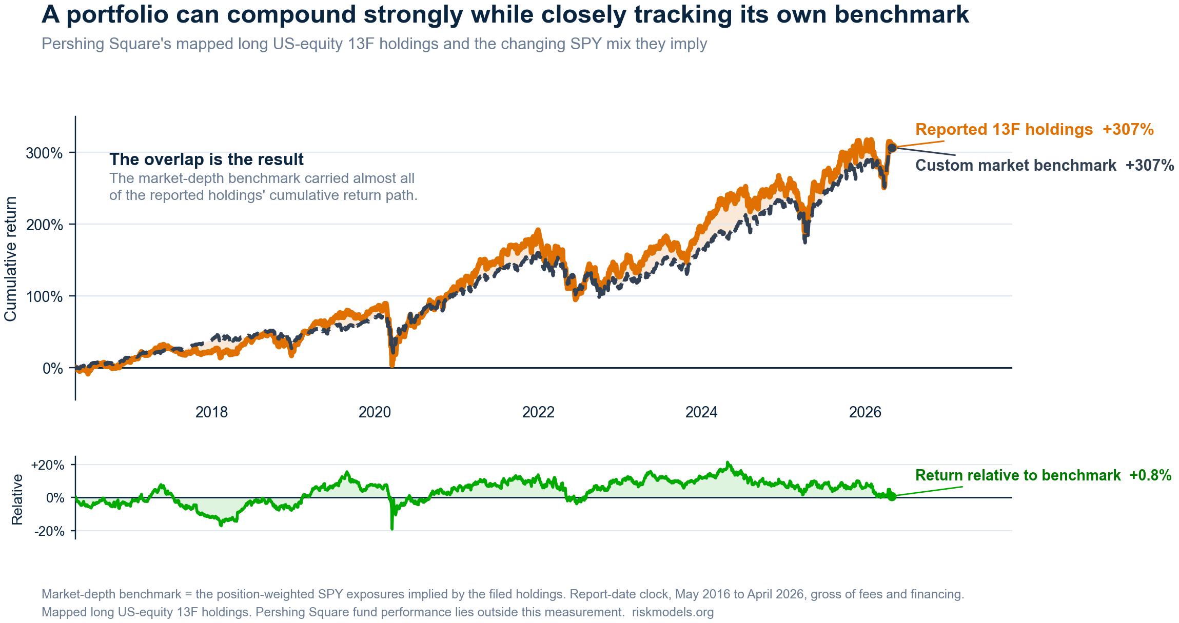
Figure 1. Cumulative return of Pershing Square's mapped long US-equity holdings reported on Form 13F, the model-implied market-depth benchmark built from their position-level SPY exposures, and the return relative to that benchmark, May 2016 to April 2026, report-date clock. Rounded endpoints are +307%, +307% and +0.8%. Returns are gross of fees and financing and represent the reported holdings rather than fund performance.
The nearly identical upper lines are the finding. Pershing's reported 13F holdings earned a high absolute return, but so did the market exposure implied by those holdings. The lower panel shows the difference.
A portfolio benchmark starts with its stocks. For NVIDIA, the ETF benchmark can stop at any of three depths:
| Benchmark depth | ETF benchmark for NVDA | Return left outside the benchmark |
|---|---|---|
| L1: Market | SPY | Sector, subsector, style and stock-specific return |
| L2: Sector | SPY + XLK | Subsector, style and stock-specific return |
| L3: Subsector | SPY + XLK + SOXX | Style and stock-specific return |
The table identifies the ETFs at each depth. The model estimates their weights afresh using information available before the return day. Adding XLK changes the SPY weight; adding SOXX changes both.
The portfolio step is arithmetic:
- Estimate the ETF weights for every stock.
- Multiply each ETF weight by that stock's weight in the portfolio.
- Add the weights of identical ETFs across positions.
NVDA and Apple can both contribute SPY and XLK legs. At portfolio level, those common exposures collapse into one SPY position and one XLK position; SOXX and RSPT remain separate subsector legs. Repeating the calculation across every holding produces one ETF benchmark for the book. Any stock portfolio with mappable constituents can be treated the same way.
The return identity is:
Portfolio return = custom ETF benchmark return + return relative to the benchmark.
The second term is often called residual or benchmark-relative return. It shows where return sits in this decomposition; it is neither total return nor a direct estimate of manager skill. High absolute return can coexist with little benchmark-relative return when the benchmark exposures also perform well.
Filed holdings supply observable stock weights. That makes it possible to build the benchmark for 2,801 portfolios, the five named filers and 144 large wealth managers. The unit of analysis is the mapped long US-equity holdings reported in each filing; the manager's full fund lies outside the filing.
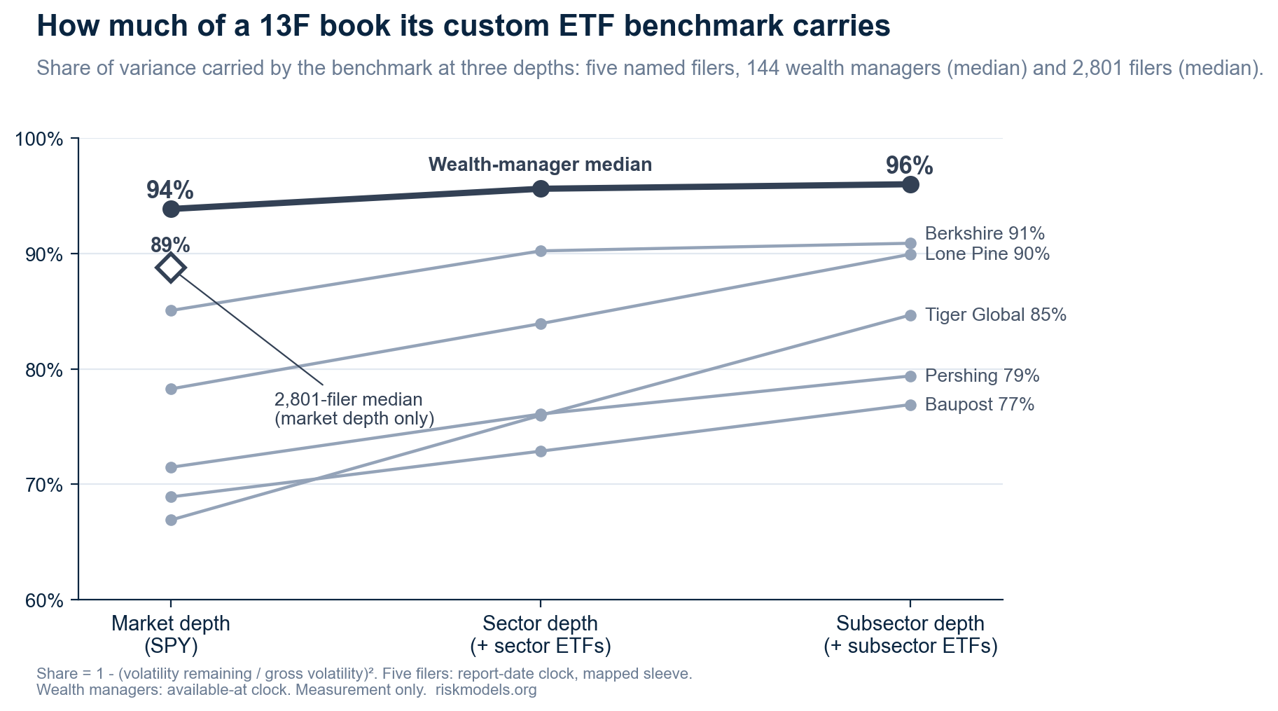
Figure 2. Share of each book's variance carried by its custom ETF benchmark at the market, sector and subsector depths: five named filers (report-date clock, May 2016 to April 2026), the median of 144 large wealth managers, and the median of 2,801 filers at market depth. The share is one minus the squared ratio of the volatility remaining after the benchmark to the gross volatility. The five filers are model-layer series, and the wealth managers are implemented series.
Tiger Global shows why benchmark depth matters. SPY alone carries 67% of its variance; sector ETFs raise the share to 76%, and subsector ETFs to 85%. The improvement comes from themes repeated across holdings: software through Microsoft, Adobe, Salesforce, ServiceNow and CrowdStrike; internet platforms through Meta, Alphabet, Sea and Reddit; retail and e-commerce through Amazon, JD.com and Carvana; and semiconductors through NVIDIA, Taiwan Semiconductor, Lam Research and Applied Materials. Berkshire begins at 85% with SPY and reaches 90% with sectors, but subsectors add only one point. Its concentrated book leaves less repeated within-sector structure for another ETF layer to capture.
Results in brief
Ten years ending April 2026. Return statistics for the five named filers and the 2,801 filers are on the report-date clock. ETF positions, turnover and wealth-manager figures begin when each filing becomes public.
Most filed equity books can be closely replicated by a compact ETF benchmark built from their own holdings. A SPY-only benchmark carries about 89% of measured variance for the median of 2,801 filers. At subsector depth, custom benchmarks carry 77% to 91% for the five named filers and about 96% for the median large wealth manager. The five named benchmarks require only 1 to 29 distinct ETFs.
Benchmark-relative return is small beside gross return in much of the sample. The median filer returned 13.8% a year gross and -0.7% relative to the market-depth benchmark. Among 100 large filers with meaningful stock-specific risk, 92 to 97 realized manager-minus-benchmark returns remain within two standard errors of zero, depending on benchmark depth.
"Factors are the language of investing that everyone should be speaking." - Andrew Ang, BlackRock
Here, small benchmark-relative returns show that market, sector and subsector exposures carried much of the measured return and most of the measured variance. The return left after those common exposures is the narrower claim on company selection, style and themes outside the traded hierarchy.
Depth has an implementation cost. Daily turnover rises as sector and subsector ETFs enter the benchmark. Monthly refresh cuts turnover to 34% to 45% of the daily rate and adds no more than 0.4 volatility points for any named filer at a fixed depth.
The filing delay has surprisingly little annual effect in most cases. Across 2,505 filers present on both clocks, market-relative returns have a rank correlation of 0.945 and a median annual change of -0.12 percentage points. Three of the five named books change by less than one point a year; Lone Pine and Tiger Global are the larger exceptions.
A 13F covers reported long US-equity holdings and omits shorts, many options, non-US positions and other assets. The results therefore describe the reported holdings rather than whole funds. The study ends before constructing an investable ETF-plus-cash return series after financing and actual trading costs.
Run the same measurement on a covered 13F filer
Install with pip install riskmodels-py, then set RISKMODELS_API_KEY to your key from riskmodels.app/get-key.
from riskmodels import RiskModelsClient

client = RiskModelsClient.from_env()
filer = "BW-FILER-CIK0001336528"  # Pershing Square
snapshot = client.get_filer_snapshot(filer)
print(snapshot)
The snapshot supplies holdings and portfolio diagnostics; decomposition fields depend on what has been materialized. It does not return the complete ten-year series or promise ETF hedge ratios. Section 8 and the API reference describe the additional calls.
Two clocks appear throughout. The report-date clock treats the quarter-end portfolio as known on that date; it is a research measure. The publicly available clock begins on the first session after filing, when a follower could trade. It is called available_at in the data. All returns are gross of fees, trading costs and financing. A filing has no daily net asset value, leaving the filer's realized fund return unavailable for comparison. Persistence lies outside this study.
1. From one stock benchmark to a portfolio benchmark
RiskModels estimates each stock's benchmark hierarchically: SPY for market exposure, a sector ETF net of market, and a subsector ETF net of both broader layers. Every estimate uses information available before the return day. Reversing the hedge signs produces the stock's long ETF benchmark. For a portfolio, multiply those ETF weights by each stock's portfolio weight and add identical ETFs across positions; exposures shared by several stocks collapse into single book-level positions. The 13F analysis uses daily-drifted portfolio weights, but the construction applies to any mappable stock portfolio.
The paper reports three fixed depths: market (SPY), sector (SPY plus sector ETFs) and subsector (SPY plus sector and subsector ETFs). Ratios are re-estimated at every depth rather than appended mechanically. The model-selected specification, L*, assigns each position its selected depth. Benchmark-relative return is book return minus benchmark return. The volatility left after the benchmark is often called tracking error; the benchmark's variance share is one minus the squared ratio of that remaining volatility to gross volatility.
The hierarchy stops at the tradability frontier. Market, sector and subsector risks can be represented with liquid ETFs. Style cannot be added as a clean fourth layer: once value, growth, quality or momentum is conditioned within a subsector, the baskets become too sparse to support stable tradable benchmarks. Style is therefore split by construction. Some travels with the sector and subsector ETFs; the rest remains in the residual. This paper chooses an observable, reproducible benchmark over a more complete but synthetic style attribution.
ETF weights need not sum to one. The benchmark consists of the ETF mix plus a cash remainder and is levered when ETF weights exceed one; reported returns exclude financing. At market depth, the SPY weight is the book's SPY beta. For Pershing Square it averages 0.95, falling to 0.44 at sector depth and 0.33 at subsector depth as more specific ETFs absorb exposure. The hedge-ratio construction removes the broader exposure already embedded in each raw ETF.
Tables 1 and 2 apply position-level ratios on the report-date clock. Table 4 aggregates the same ratios into book-level ETF positions after each filing becomes public. Differences between the model components and aggregated ETF positions are implementation diagnostics and are reported outside the main argument.
The benchmark locates the return and risk carried by the filed book. The residual after subsector depth includes company-specific return, style and any themes the traded hierarchy does not capture; it is not, by itself, an estimate of manager skill.
2. For the median filer, the market-depth benchmark carries about 89% of variance
The analysis begins with daily holdings-based returns for 15,333 filers. After applying the history, coverage, breadth and sanity requirements, 2,801 have the ten-year histories reported in Table 1.
| Item | Value |
|---|---|
| Filers with a daily return series in the store | 15,333 |
| With at least 80% of business days usable, May 2016 to April 2026 | 3,112 |
| After mapped coverage of at least 80%, at least five names, and a sanity filter on return and volatility | 2,801 |
| Filers meeting the same rules for May 2021 to April 2026 | 4,705 |
| Reported 13F value of the 2,801 (latest filing; includes overlaps between parents and sub-advisers) | $53.7 trillion; median $0.96 billion (10th to 90th percentile $0.19 to $14.5 billion) |
| Annualized gross return, median | 13.8% |
| Annualized return from the book's SPY beta, median | 14.9% |
| Return relative to the market-depth benchmark (SPY-hedged), median; 5th / 25th / 75th / 95th percentile | -0.7%; -6.5% / -2.2% / +0.4% / +3.0% |
| Median relative to the sector-depth benchmark; relative to the subsector-depth benchmark (stock-specific layer) | 0.0%; +0.5% |
| Filers with a positive return relative to the market-depth benchmark | 34% |
| Median share of layer variance: market / sector / subsector / stock-specific | 90% / 2% / 1% / 6% |
| Median volatility, gross and relative to the market-depth benchmark | 19.0% and 6.3% |
Table 1. The 2,801 filers with ten-year histories, May 2016 to April 2026, report-date clock, model-layer series. Medians across filers unless stated; returns annualized. The SPY-hedged return is the return relative to the market-depth benchmark.
The median filer returned 13.8% a year gross. The return associated with the SPY betas of its positions was 14.9% a year, and the return relative to that market-depth benchmark was -0.7%. As separate cross-sectional medians, their sum has no interpretation. The positive relative-return share was 34%. Market exposure accounted for 90% of layer variance for the median filer, and benchmarking that exposure reduced volatility from 19.0% to 6.3%.
Requiring ten years creates survivorship bias by excluding filers that closed after 2016. Among filers observed in 2016-2021, those absent in 2021-2026 had a median first-window relative return of -0.61% a year, versus -0.37% for survivors. Their positive shares were 41% and 44%. The reported -0.7% median and 34% positive share therefore modestly overstate the full population. Appendix I compares gross and relative-return ranks.
3. Realized manager-minus-benchmark returns cluster near zero across 100 large filers with material stock-specific risk
The five named filers are recognizable examples, but they are too small a sample to establish the distribution. Figure 3 expands the test to the 100 largest ten-year filers whose stock-specific layer carries at least 10% of variance. The screen uses risk, not realized benchmark-relative return, and is an operational definition of active risk rather than a legal classification of the manager.
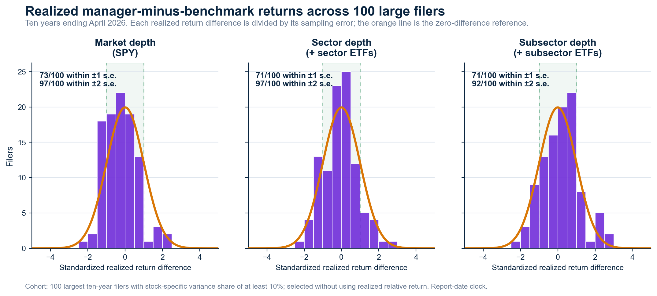
Figure 3. Realized ten-year benchmark-relative returns divided by their sampling errors for 100 large filers with material stock-specific risk, May 2016 to April 2026, report-date clock. The filers are the 100 largest by reported 13F assets among the ten-year sample with at least 10% stock-specific variance. The orange line is the marginal distribution expected if the true benchmark-relative return is zero; the three depths for a filer are not independent.
At market depth, 73 of 100 realized differences lie within one standard error of zero and 97 lie within two. The corresponding counts are 71 and 97 at sector depth, and 71 and 92 at subsector depth. The distribution shifts slightly as the benchmark becomes more specific, but most realized return differences remain small relative to their sampling error at every depth.
The five named filers show how individual books sit inside that broader result.
Pershing's return relative to its subsector-depth benchmark is +1.9% a year, with a standard error of 3.0 points
| Filer | Gross | Relative to market-depth benchmark (SE) | Relative to sector-depth benchmark (SE) | Relative to subsector-depth benchmark, stock-specific (SE) | Volatility, gross to relative (market depth) | Max drawdown, gross / relative (market depth) | Rank, gross / relative (market depth) |
|---|---|---|---|---|---|---|---|
| Berkshire Hathaway | +13.5% | −1.3% (2.5) | −1.1% (2.0) | −1.4% (1.9) | 20.4% to 7.9% | −39.3% / −20.7% | 1,576 / 1,771 |
| Lone Pine Capital | +16.9% | −0.2% (3.7) | −0.9% (3.2) | −0.3% (2.5) | 25.0% to 11.7% | −52.9% / −43.0% | 368 / 1,095 |
| Tiger Global | +18.9% | +1.6% (5.1) | +0.6% (4.4) | +2.2% (3.5) | 28.2% to 16.2% | −65.0% / −59.7% | 175 / 310 |
| Pershing Square | +15.1% | +0.1% (3.6) | −0.1% (3.3) | +1.9% (3.0) | 21.0% to 11.2% | −45.5% / −30.1% | 782 / 912 |
| Baupost Group | +5.1% | −9.9% (4.0) | −9.1% (3.8) | −7.4% (3.5) | 22.8% to 12.7% | −47.7% / −68.6% | 2,743 / 2,741 |
Table 2. Five filers, annualized, May 2016 to April 2026, report-date clock, model-layer series, mapped long 13F holdings only. Each return column is the return relative to the benchmark at that depth. Mean mapped weight coverage is 98% for Berkshire, 97% for Lone Pine, 96% for Pershing Square, 91% for Tiger Global and 84% for Baupost (Appendix F). Standard error is the volatility of each relative-return series divided by the square root of ten years. Ranks are among the 2,801 filers.
Depth determines which exposures enter the ETF mix and which remain. Pershing Square realized +0.1% a year relative to the market benchmark, -0.1% relative to sector and +1.9% relative to subsector. With annual relative volatility near 10%, the ten-year standard errors are about three points. None of Pershing's realized differences is distinguishable from zero or from the others. The same is true for Tiger Global (+1.6%, +0.6% and +2.2%) and Berkshire Hathaway (-1.3%, -1.1% and -1.4%).
Figure 1's 307% cumulative gross return and 0.8% cumulative market-relative return answer different questions. The first reconstructs the reported long-equity holdings. The second shows that a changing SPY mix, sized from those holdings' measured market exposure, earned almost the same daily return. Neither series is the fund's net asset value: the filing omits shorts, many options, non-US positions and other assets.
Baupost is the only named filer more than two standard errors from zero: -9.9% a year relative to market, with a 4.0-point standard error, and -7.4% relative to subsector, with a 3.5-point standard error. The mapped holdings cover 84% of filed value; the rest of Baupost's portfolio lies outside the analysis.
For an allocator, the comparison separates common thematic exposures from the return left for company selection and unmodeled risks. Managers who own different stocks may still share those exposures. Section 6 then tests how much return survives the wait for a public filing.
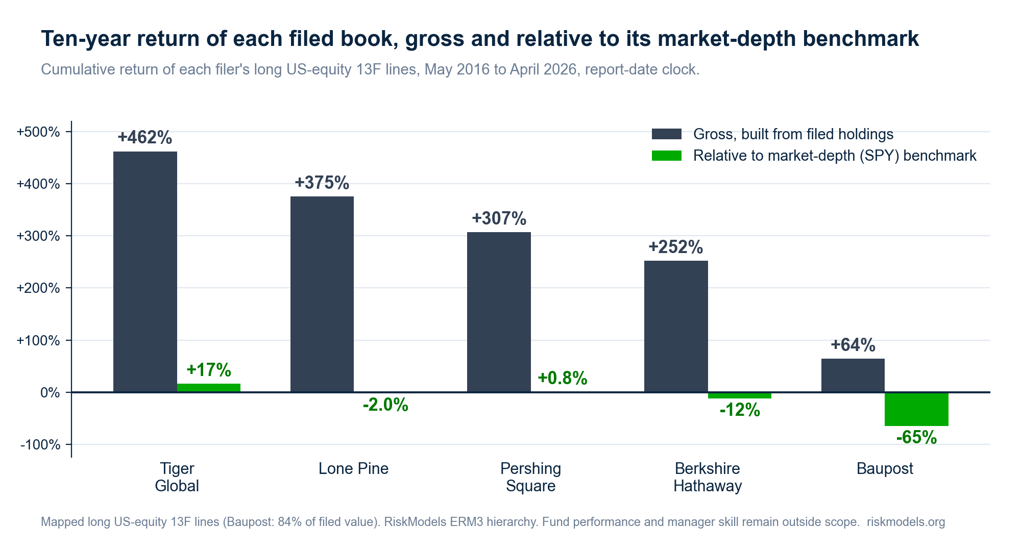
Figure 4. Cumulative return of each filer's long US-equity 13F lines, gross and relative to its market-depth benchmark, May 2016 to April 2026, report-date clock. These returns come from filed holdings rather than fund net asset values: the 13F excludes non-equity positions, and Baupost's mapped coverage is 84% of filed value.
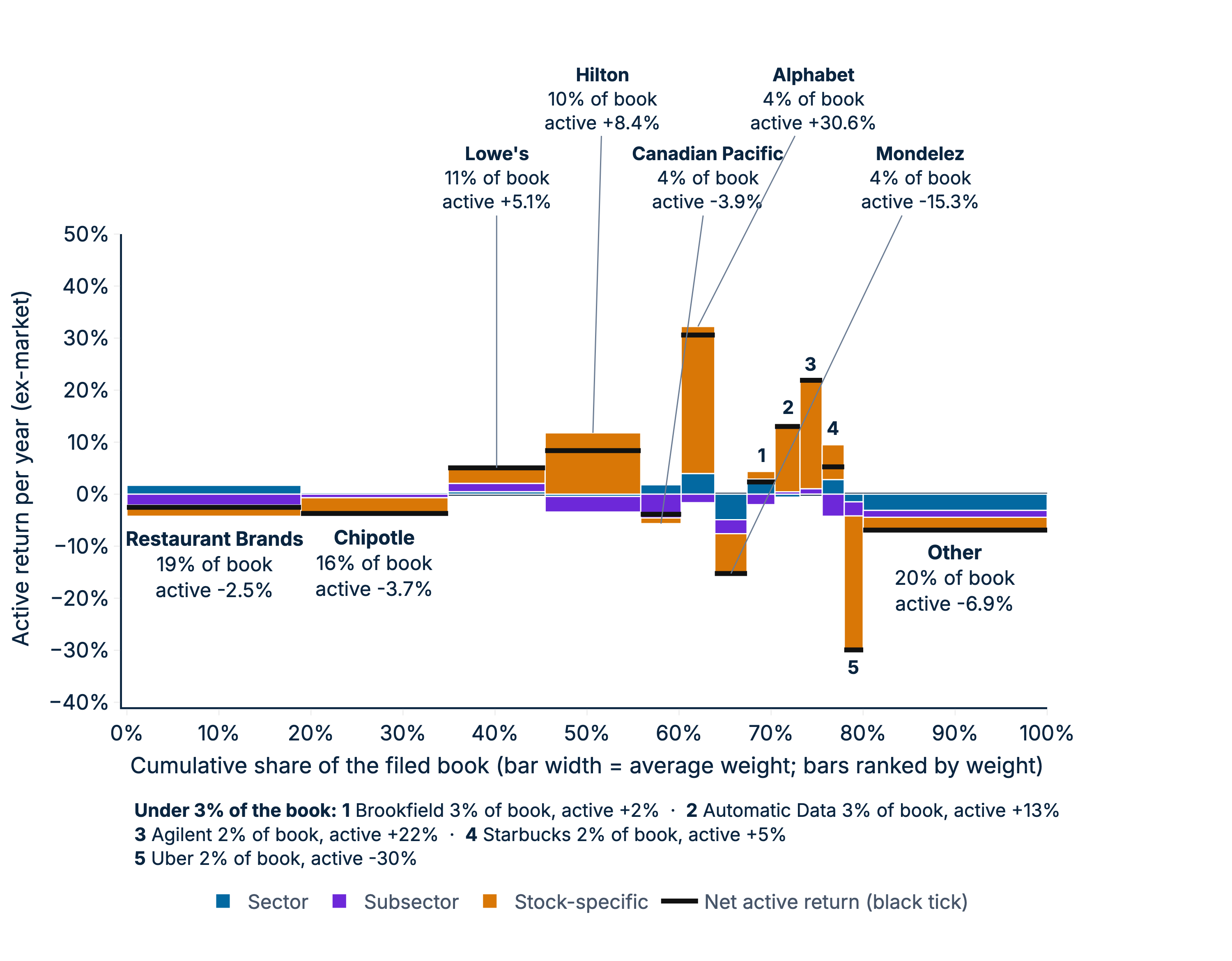
Figure 5. Pershing Square by stock, market layer removed, May 2016 to April 2026. Bar width is the stock's average weight in the whole mapped book, height is its annualized return while held split into sector, subsector and stock-specific layers, and the black tick is the net. Bars are ordered by weight; issuers under 1.5% of the book are pooled as Other holdings.
The stock cascade locates Pershing's remaining return. Over ten years, Hilton Worldwide contributes +28.0 points, Chipotle +20.5 and Alphabet +28.2 across its two listings. Uber contributes -15.7, Howard Hughes -22.0 across two entities and Netflix -9.3. The subsector layer contributes -40.0 points, including -19.5 from the leisure and entertainment cohort containing Hilton, Restaurant Brands and Chipotle.
Pershing's realized difference changes sign across depths, yet all three values remain within one standard error of zero. Appendix D reports Berkshire Hathaway's sector cascade: technology contributes about 5 points a year of ex-market return, while consumer staples and financials each contribute about -4 points.
4. For 144 large wealth managers the subsector-depth benchmark carries about 96% of variance
The wealth-manager books are broader and more diversified. The median adviser reports 683 13F lines. Directly held model stocks cover 39% of filed value at the median and 62% after looking through funds and ETFs. Results refer only to those covered long US-equity holdings. Of the 144 advisers with at least 500 return days, 74 have the full May 2016 to April 2026 history; the shortest history contains 553 days. Appendix G defines the Form ADV cohort and reports look-through, concentration and style.
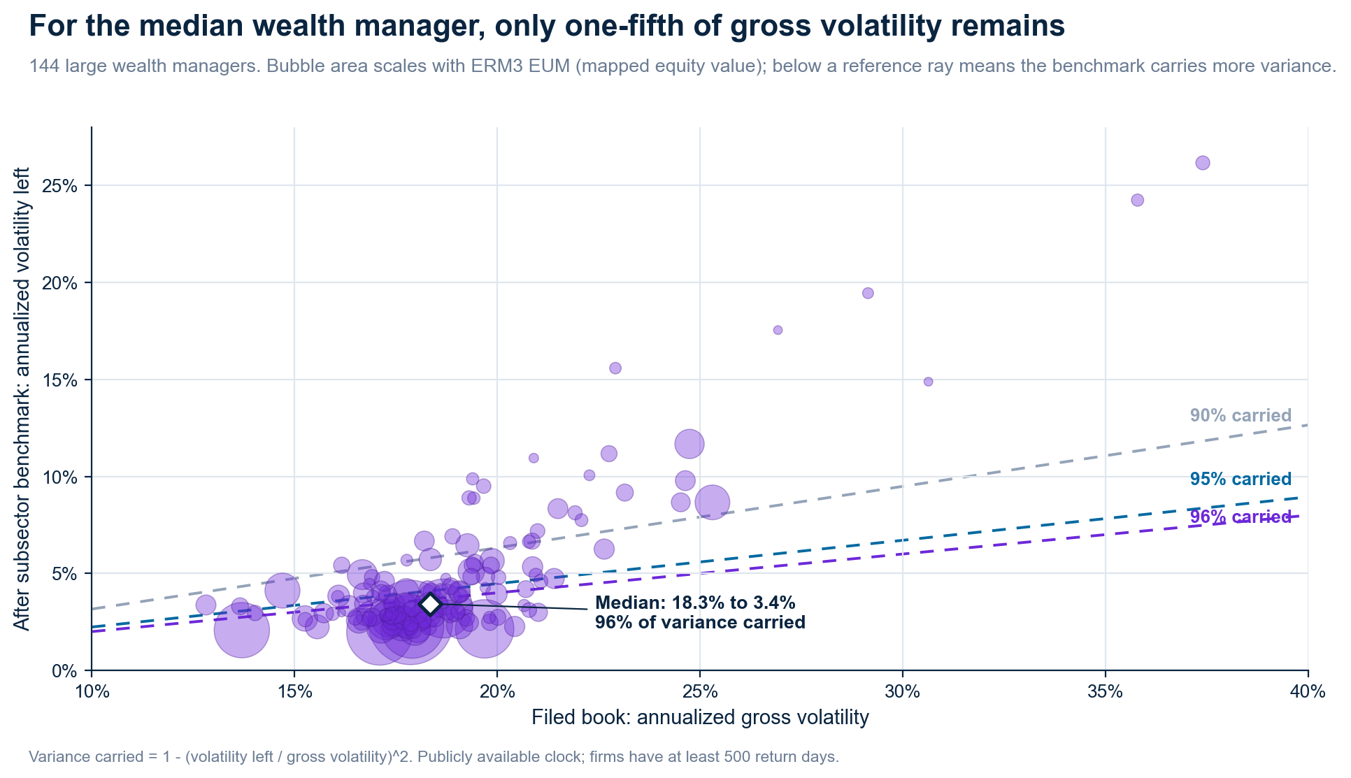
Figure 6. Annualized gross volatility against volatility left after the subsector-depth benchmark, daily refresh, publicly available clock, 144 advisers with at least 500 return days. Bubble area scales with ERM3 EUM (mapped equity value). The reference rays show where the benchmark carries 90%, 95% and 96% of variance; points below a ray have a higher benchmark share.
Median annualized gross volatility is 18.3%, with quartiles of 17.3% and 19.8%. Market depth leaves 4.4% volatility and 6.1% of variance at the median of the per-firm ratios, so the benchmark carries 94%. Sector depth leaves 3.7% volatility and 4.4% of variance. Subsector depth leaves 3.4% volatility and 4.0% of variance: a 96% benchmark share. The scatter shows that this is not only a median result: 114 of 144 managers have at least 90% of variance carried by the benchmark, and 84 have at least 95%. The remainder includes company-specific return, style and themes outside the traded hierarchy.
The median adviser holds ten of eleven sectors at weights of at least 1%, eight at weights of at least 3%, and 36% in the largest sector; the quartiles are 31% and 41%. Sector depth reduces median volatility by 0.8 points beyond SPY. Subsector depth removes another 0.2 points, based on unrounded medians of 4.45%, 3.65% and 3.43%. The causal link between sector breadth and the smaller gain at the final depth remains untested.
| Benchmark depth | ETFs | Volatility left, % (daily) | Relative return, % | Turnover D / W / M | Cost, bp of book: daily / monthly |
|---|---|---|---|---|---|
| Filed book | - | 18.3% (17.3, 19.8) | 13.5% (12.3, 15.1) | - | - |
| Market depth (SPY) | 1 (1, 1) | 4.4% (3.2, 6.9) | -0.6% (-1.6, 0.4) | 0.9/0.6/0.3 | 0.9/0.3 |
| Sector depth | 12 (11, 12) | 3.7% (2.6, 5.6) | 0.5% (-0.4, 1.2) | 3.4/2.1/1.2 | 3.4/1.2 |
| Subsector depth | 33 (29, 35) | 3.4% (2.7, 5.4) | 1.0% (0.2, 1.6) | 6.6/4.6/2.4 | 6.6/2.4 |
| Model-selected level (L*) | 19 (16, 21) | 4.0% (3.1, 5.8) | 0.8% (-0.1, 1.4) | 7.3/6.1/2.6 | 7.3/2.6 |
Table 3. Cohort medians with 25th and 75th percentiles in parentheses, 144 advisers with at least 500 return days, publicly available clock, before financing and differences between ETF and index returns. Turnover in multiples of book per year; cost at 1 basis point per unit traded.
The median annualized gross return is 13.5%. Median return relative to the benchmark is -0.6% at market depth, +0.5% at sector depth, +1.0% at subsector depth and +0.8% at the model-selected depth. The interquartile range is 1.4 to 2.0 points wide at each depth. The 1.6-point span between the lowest and highest depth medians is therefore similar to the cross-sectional spread between advisers at a single depth.
For an RIA, the practical result is a benchmark of about 33 ETFs for a covered client book with hundreds of lines. It provides a common basis for comparing accounts and explaining their exposures within an existing reporting system. The results cover each adviser's available history and precede costs, financing and differences between ETF and index returns.
5. The benchmark is compact, but it is not static
At portfolio level, the same ETFs recur across many holdings. Combining those exposures turns the stock-by-stock benchmark into a short ETF list. Market depth requires only SPY. Sector depth requires 7 to 11 ETFs for the five named filers and 12 for the median wealth manager. Subsector depth requires 16 to 29 for the named filers and 33 for the median wealth manager. A portfolio with many stocks can therefore be benchmarked with a few dozen traded instruments.
Table 4 reports the ETF count, volatility left after the benchmark, relative return, turnover and illustrative cost for the five named filers on the publicly available clock. Table 3 gives the corresponding wealth-manager results. An ETF counts when its mean absolute weight over the measured history exceeds 0.5%.
| Filer | Benchmark depth | ETFs | Volatility left (D) | Relative return | Turnover (D / M) | Cost, bp (daily) |
|---|---|---|---|---|---|---|
| Pershing Square | Filed book | - | 20.9% | +15.0% | - | - |
| Market depth (SPY) | 1 | 11.2% | 0.0% | 1.2 / 0.5 | 1.2 | |
| Sector depth | 9 | 10.3% | +0.5% | 4.7 / 2.1 | 4.7 | |
| Subsector depth | 16 | 9.5% | +2.3% | 7.9 / 3.4 | 7.9 | |
| Model-selected level (L*) | 14 | 9.7% | +1.3% | 8.8 / 3.3 | 8.8 | |
| Berkshire Hathaway | Filed book | - | 20.5% | +13.1% | - | - |
| Market depth (SPY) | 1 | 7.9% | −1.6% | 1.0 / 0.4 | 1.0 | |
| Sector depth | 9 | 6.4% | −1.1% | 4.6 / 1.6 | 4.6 | |
| Subsector depth | 21 | 6.2% | −1.4% | 8.8 / 3.3 | 8.8 | |
| Model-selected level (L*) | 11 | 7.0% | −1.2% | 9.8 / 4.0 | 9.8 | |
| Tiger Global | Filed book | - | 28.0% | +16.0% | - | - |
| Market depth (SPY) | 1 | 16.4% | −0.8% | 1.9 / 0.8 | 1.9 | |
| Sector depth | 7 | 14.3% | −0.7% | 6.3 / 2.2 | 6.3 | |
| Subsector depth | 21 | 11.3% | +1.1% | 10.7 / 4.1 | 10.7 | |
| Model-selected level (L*) | 15 | 12.8% | +0.3% | 12.5 / 4.3 | 12.5 | |
| Lone Pine | Filed book | - | 24.8% | +15.1% | - | - |
| Market depth (SPY) | 1 | 11.9% | −1.5% | 1.5 / 0.5 | 1.5 | |
| Sector depth | 11 | 10.4% | −0.9% | 5.7 / 2.1 | 5.7 | |
| Subsector depth | 29 | 8.1% | +0.6% | 10.7 / 4.4 | 10.7 | |
| Model-selected level (L*) | 20 | 9.1% | 0.0% | 12.1 / 4.3 | 12.1 | |
| Baupost | Filed book | - | 21.7% | +4.8% | - | - |
| Market depth (SPY) | 1 | 12.3% | −9.0% | 1.6 / 0.6 | 1.6 | |
| Sector depth | 11 | 12.2% | −5.8% | 5.2 / 1.9 | 5.2 | |
| Subsector depth | 27 | 12.0% | −4.2% | 13.5 / 5.3 | 13.5 | |
| Model-selected level (L*) | 17 | 12.2% | −5.1% | 7.8 / 2.7 | 7.8 |
Table 4. ETF positions that implement each benchmark depth for five filers, aggregated from per-stock ratios, filings credited from the first session after the filing date (publicly available clock), May 2016 to April 2026. Return is annualized and gross of financing and differences between ETF and index returns. Turnover is in multiples of book per year; cost is turnover at 1 basis point per unit traded.
More detail improves the match, but it also increases trading. With daily refresh, the subsector benchmark turns over 7.9 to 13.5 times the book each year for the five named filers and 6.6 times for the median wealth manager. At the paper's illustrative cost of one basis point per unit traded, those turnover figures translate to 7.9 to 13.5 basis points a year for the named filers and 6.6 basis points for the median wealth manager. These estimates exclude bid-ask spreads, financing and differences between ETF and index returns.
Pershing Square shows what the extra detail buys. Volatility left after the benchmark falls from 11.2% with SPY alone to 9.5% with the subsector benchmark. Its annual return relative to the benchmark changes from 0.0% at market depth to +0.5% at sector depth and +2.3% at subsector depth. Each result remains inside its roughly three-point standard error. The deeper benchmark changes the explanation of Pershing's return, but not the statistical conclusion.
L* makes a different choice for each stock: it stops at market, sector or subsector depth according to the model's selected level. That reduces the median wealth manager's ETF list from 33 to 19 and the named filers' lists from 16-29 to 11-20. It does not reduce trading. At the median, L* turns over 7.3 times the book with daily refresh, compared with 6.6 times for the fixed subsector benchmark, and leaves 4.0% rather than 3.4% volatility unexplained. L* is therefore a smaller but less stable ETF mix, not a uniformly cheaper one.
Monthly refresh preserves the match while cutting ETF turnover by about two-thirds
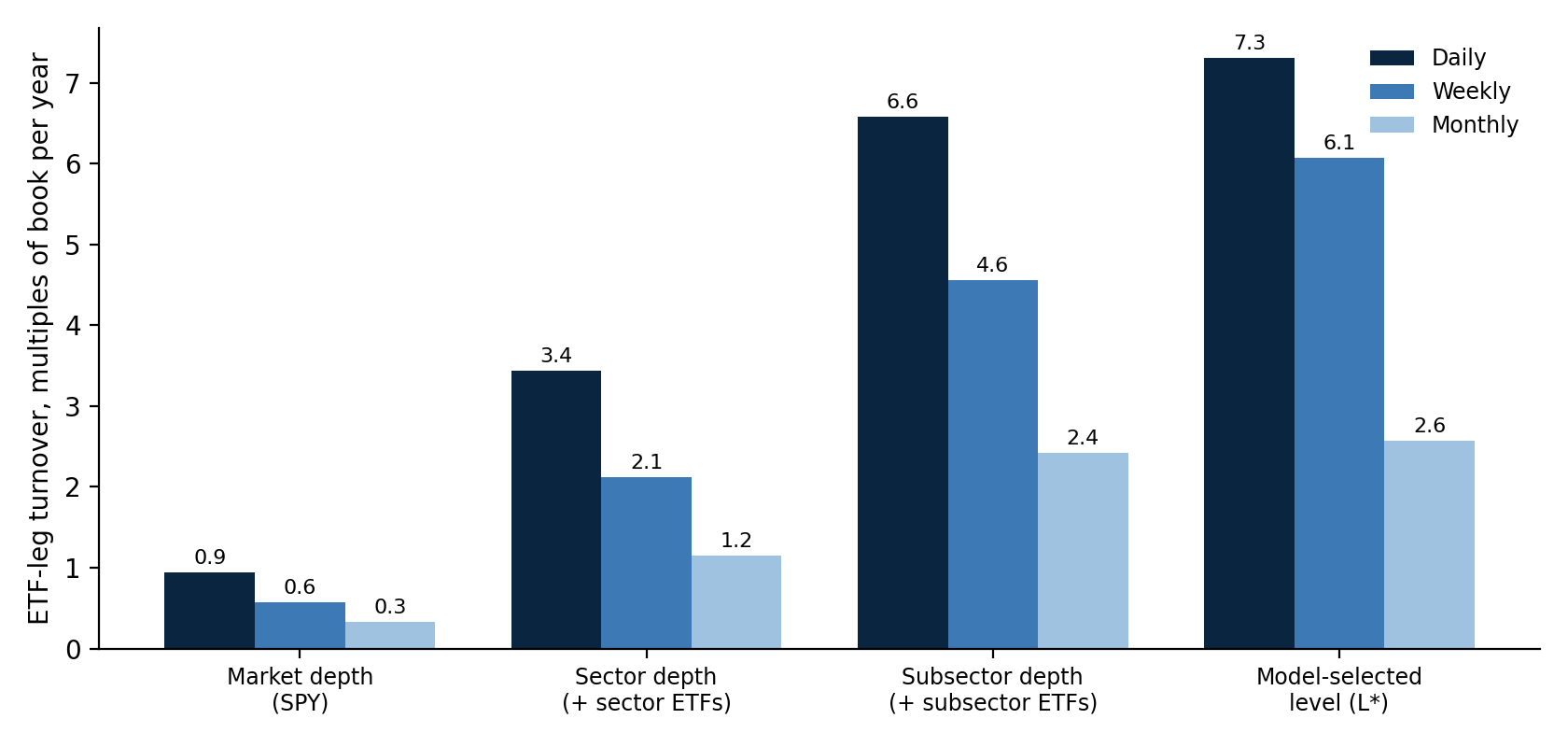
Figure 7. Median turnover of the ETF benchmark, in multiples of book per year, at daily, weekly and monthly refresh with weights frozen between refreshes. The median ETF counts are 1 at market depth, 12 at sector depth, 33 at fixed subsector depth and 19 for L*. Fewer ETFs does not imply lower turnover. 144 wealth managers.
Monthly refresh reduces median subsector turnover from 6.6 to 2.4 times the book and L* turnover from 7.3 to 2.6. The median increase in unexplained volatility is only 0.05 to 0.14 percentage points across depths; for every named filer it is no more than 0.4 points. Monthly refresh captures most of the benchmark's explanatory value with roughly one-third of the daily trading.
The practical point is simple. Shared ETF exposures combine across holdings into a short benchmark portfolio. The return left after that benchmark belongs to the individual stocks, style and themes outside the hierarchy rather than to the market, sector and subsector exposures they share.
6. Public filings preserve most of the reported book's return
A 13F becomes public as much as 45 days after quarter-end. To test whether that delay defeats a holdings-based strategy, the analysis runs each reported book on two clocks. The first applies a filing at quarter-end, before an investor could know it. The second begins on the first trading session after the filing becomes public. The difference is the return effect of waiting for information an investor could actually use.
For the 2,505 filers present on both clocks, market-relative annual returns have a rank correlation of 0.945. The median change is -0.12 percentage points a year. Waiting for the public filing therefore usually preserves both the manager's relative standing and most of the return measured from the reported long book.
The five named filers show the range of outcomes. Berkshire Hathaway changes from 13.46% to 12.54% a year, Pershing Square from 15.10% to 15.95%, and Baupost from 5.10% to 5.58%. Lone Pine falls by 1.60 points a year and Tiger Global by 1.80 points. Those two are material exceptions, but even there the public holdings retain most of the book's annual return.
This makes the public filing useful for following the disclosed portfolio. It does not reproduce the manager's fund return: 13Fs omit shorts, cash, non-US securities and most derivatives, and the calculation is gross of fees and trading costs. The narrower conclusion is still important. For most filers, an investor who waits until the holdings are public can follow the reported long US-equity book without losing its basic return profile. The stock-specific risk share moves by no more than two points for the five named filers, a secondary confirmation that the delay does not materially alter the measured structure.
7. Scope, limitations, and next tests
The sample covers long US-equity 13F lines that map to the model universe from May 2016 to April 2026. Returns are gross of fees, financing and differences between ETF and index returns. Table 2 standard errors assume independent daily relative returns. The cost calculation charges every ETF 1 basis point per unit traded, including thin subsector funds, so the cost columns simply restate turnover under that assumption.
The wealth-manager cohort relies on self-reported Form ADV fields and excludes firms with blank CIKs. Direct model stocks cover a median 39% of filed value and 62% after fund look-through. Every wealth-manager return and volatility statistic refers to that covered portion of the reported holdings.
Filer record for Pershing Square. Pershing Square Capital Management (CIK 0001336528) is flagged stopped_filing in the filer master because its latest filing is for 31 March 2026, one quarter before the latest quarter in the store. A second filer, Pershing Square Inc. (CIK 0002026053), has filings for 30 June 2025 through 30 June 2026, so the two filed in parallel for four quarters. The filer master lacks a succession record, this analysis leaves the relationship unresolved, and the ten-year series covers the capital-management filings only. EDGAR (checked 14 November 2026) lists Pershing Square Inc. under that name since 23 April 2026, formerly Pershing Square Holdco, L.P., and shows a 13F notice (form 13F-NT) rather than a holdings report from Pershing Square Capital Management for 30 June 2026.
The next tests are:
- The return and volatility of the long ETF mix plus its cash remainder on its own, after each filing becomes public, at daily and monthly refresh, for the five filers and the 144 advisers.
- Placebos for the depth results: a benchmark built with each filer's own-history OLS beta and one built with a beta of one to SPY.
- Financing and ETF bid-ask costs in the leg-cost estimate, using the ETFs' own spreads.
- The same table for 20 to 30 additional named filers, extending the named evidence beyond the five cases reported here.
8. How a reader runs the same measurement
RiskModels.org is the open research and methodology reference: the ERM3 specification, published papers and visual dossiers. RiskModels.app is the production API engine. Install the Python SDK with pip install riskmodels-py, use REST or the CLI, or connect an agent through MCP. Self-service access is billed per successful call, with $20 in free starter credits after card setup and no subscription or seat fees; current terms are on the pricing page.
An allocator can compare managers' common thematic exposures, the return left after those exposures, and the return lost while waiting for public filings. An RIA can construct a benchmark for a client book with hundreds of lines: the median wealth-manager benchmark here uses 33 ETFs at subsector depth. The same measurement can sit in an existing reporting stack. Developers can use the structured, point-in-time model output as a deterministic quantitative input to code or an agent, retaining the dates, coverage and model version returned with each response.
RiskModels provides portfolio measurement rather than order execution. For a stock, get_hedge_basket returns the L* ETF legs as signed ratios per $1 of stock. get_alpha, with depth set to L1, L2 or L3, returns fixed-depth legs. For a list of positions, analyze_portfolio returns layer attribution and portfolio hedge ratios. Weight the stock-level legs and aggregate them by ETF to form the book-level benchmark.
Select a covered 13F filer through the RiskModels API to retrieve its disclosed holdings and the returns calculated from those holdings. get_filer_holdings returns the latest-quarter holdings and get_filer_concentration returns concentration measures. Return attribution accepts portfolios of up to 100 stocks, and longer return histories can be assembled through the API. The results can be returned directly to an agent or integrated into a research or production code stack.
Coverage includes daily holdings-based return series for 15,333 filers keyed by bw_filer_id, which embeds the CIK. Parent filers, sub-advisers and funds of funds can overlap. No single call returns the complete ten-year series. The API reference is at riskmodels.app/docs/api; keys are issued at riskmodels.app/get-key.
Appendices A to I are in the PDF version of this paper.