
Cascade Hedging and the Cost of Interpretability
Subsector ETF value, joint optimization, and executable hedge layers across 9,074 US mutual funds
Conrad Gann · Blue Water Macro · Working Paper · May 2026
Abstract. We compare three out-of-sample hedge constructions for US mutual funds: sector-only principal-component regression (PCR) on eleven GICS sector ETFs (a common transparent practitioner baseline); a hierarchical cascade with orthogonalized market, sector, and subsector layers; and joint PCR on a curated 68-ETF panel (1 market + 11 sector + 56 subsector). Using paired monthly evaluations for 9,074 funds from April 2020 through April 2026, we map where subsector hedging value resides and how much a structured estimator captures relative to joint optimization on the fit–stability–executability frontier.
Subsector ETFs add incremental information beyond sector baskets for most funds. The cascade improves on the practitioner baseline while trailing joint PCR by a comparable margin—the cost of interpretability: executable per-layer notionals and hierarchical attribution rather than a single joint basket. Among funds with meaningful subsector value, median cascade extraction efficiency is 0.45, with wide cross-fund dispersion. Joint PCR is numerically stable within this universe but exhibits roughly three times the coefficient drift of the cascade; unconstrained joint OLS is singular for every fund. Tail robustness checks leave signed conclusions unchanged.
JEL: G11, G23, C58 · Keywords: hedge ratios, ETF replication, factor models, mutual funds, out-of-sample evaluation
1. Introduction
Mutual-fund risk teams routinely ask whether a fund's return can be replicated out of sample by a basket of liquid ETFs. The question has grown more operational in the past decade: industry and thematic ETF suites now span GICS subsectors, and Form N-PORT gives researchers and vendors holdings-level panels to reconstruct fund-equivalent returns at scale. Outside licensed commercial models (e.g., Barra, Axioma), the standard answer still regresses fund returns on broad-market and GICS sector ETFs—often with principal-component regularization to handle mild collinearity within the sector block.
That practice leaves two structural questions open. First, do subsector ETFs carry incremental hedging information beyond eleven sector funds? Second, if they do, how much can a structured estimator recover when the deliverable must include stable, layer-attributed hedge notionals—not only a single joint basket tuned for raw fit?
This paper answers both with a matched three-way out-of-sample census. We reconstruct daily fund-equivalent returns from N-PORT holdings for 9,074 US mutual funds and, at each date on a common monthly grid, fit three constructions on identical training windows: sector-only PCR, a hierarchical cascade with sequential orthogonalized layers, and joint PCR on the full 68-ETF universe (1 + 11 + 56). Per-fund paired gaps decompose total subsector value, cascade capture, and the residual to joint optimization—holding fund, date, and window fixed.
Three estimator questions (plain English). Sector-only hedging asks: Can broad sector ETFs explain the fund? Joint PCR on the curated 68-ETF universe asks: What is the best statistical ETF basket if reporting structure is ignored? The cascade asks a different product question: How much of the same ETF information can be recovered while preserving market, sector, and subsector hedge layers that can be reported, audited, and traded separately? The paper measures where those three answers diverge on the fit–stability–executability frontier—not which estimator "wins" on R² alone.
Contribution. Prior work establishes shrinkage and structured covariance estimation (Ledoit and Wolf; POET; instrumented PCs) and documents backtest overfitting in finance (Harvey, Liu and Zhu). We add a population-scale paired decomposition: where L3 ETF value lives, how much a cascade extracts (via extraction efficiency), and what joint optimization buys in R² at the cost of stability and executability. Joint PCR fits better on median OOS R² within our curated universe; the cascade earns its place by occupying a defensible point on that frontier.
Three regularities organize the results. Subsector ETFs matter for a large share of the cross-section—not uniformly, but far from negligible. The cascade materially improves on sector-only practice while surrendering roughly as much to joint PCR as it gains over the baseline; extraction efficiency quantifies that partition. Joint PCR's fit advantage pairs with materially higher coefficient drift; unconstrained joint OLS is non-invertible throughout every fund's history.
Sections 2–6 situate the estimators (§2), describe data and methods (§3), present results (§4), discuss implications (§5), and conclude (§6).
2. Related Work
We organize prior work into three strands that bound our comparison.
2.1 Covariance shrinkage and conditioning
Ledoit and Wolf (2003, 2004) formalize bias–variance tradeoffs in large-dimensional covariance estimation; Engle, Ledoit and Wolf (2019) extend the framework to dynamic settings. Jorion (1986) and James and Stein (1961) anchor empirical-Bayes portfolio estimation. Our sector-only and joint PCR baselines apply Stock and Watson (2002) principal-component regression to ETF panels—standard regularization when collinearity is mild (eleven sectors) or severe (68 ETFs jointly). The cascade adds sequential orthogonalization and Vasicek shrinkage on underlying stock betas (Vasicek 1973; see §3.3 note).
2.2 Hierarchical and structured factor models
Fan, Liao and Mincheva (2013) estimate large covariances via POET; Kelly, Pruitt and Su (2019) and Lettau and Pelger (2020) estimate latent factors with eigenvalue shrinkage. Fama and French (1993) provide the low-dimensional template sector-ETF regressions approximate. Avellaneda and Lee (2010) extract latent factors from stock return matrices for statistical arbitrage—the closest ancestor of our joint full-ETF view, transplanted to tradable ETFs. López de Prado (2016) applies hierarchical structure to portfolio construction (risk parity). The cascade is a parametric hierarchical model with explicit ETF legs; joint PCR is the non-parametric latent-factor benchmark on the same tradable universe.
2.3 Out-of-sample discipline and holdings-based context
Harvey, Liu and Zhu (2016) and López de Prado (2014) document backtest overfitting; all metrics here use 60-day OOS holdouts from a rolling production design, with coefficient drift reported alongside R². Cremers and Petajisto (2009) measure benchmark deviation via active share; the cascade's per-layer ETF notionals are compatible with holdings-attributed reporting from N-PORT, though we do not pursue that integration here.
3. Data and Methodology
3.1 Universe and return construction
The sample comprises US mutual funds in the ERM3 fund registry with holdings-reconstructed daily returns and precomputed hedge diagnostics for all three views. Of 9,649 registry funds, 9,074 (94%) enter the paired analysis: each has at least six monthly evaluation dates with finite out-of-sample R² in every view.
For each fund, the target series is the daily holdings-reconstructed gross return on an as-filed (report_date) lag basis—the same basis used for stored cascade and joint-PCR benchmarks. The tradable factor panel contains 68 ETFs in three layers: 1 broad-market fund (SPY), 11 GICS sector SPDRs, and 56 industry subsector ETFs (1 + 11 + 56 = 68). Holdings panels begin with the N-PORT era (April 2019 onward); ETF histories extend to May 2006 for rolling training depth.
3.2 Sample window and observation counts
Table 1 summarizes the evaluation design. Per-fund headline statistics aggregate across the median of 25 qualifying monthly evaluations, then across funds.
Table 1. Sample window and observation counts
| Item | Value |
|---|---|
| Fund registry (universe) | 9,649 |
| Paired analysis sample | 9,074 (94%) |
| Qualifying rule | ≥ 6 monthly eval dates; finite OOS R² in all three views |
| Median paired eval dates per fund | 25 (max 25 in census) |
| Monthly evaluation grid | 2020-04-30 → 2026-04-30 (73 endpoints per fund) |
| Training window | 1,260 trading days ending at each eval date |
| OOS holdout | 60 trading days immediately after training |
| Minimum training history | 252 trading days |
| Holdings coverage era | 2019-04-01 onward |
| ETF panel span | 2006-05-22 → 2026-05-22 |
3.3 Three hedge constructions
At each monthly evaluation date, each construction fits on a 1,260-day training window and evaluates R² on the subsequent 60-day holdout (minimum 252 training days).
(a) Sector-only PCR (practitioner baseline). PCR with 95% cumulative-variance component selection, capped at min(20, p − 1) = 10 components on the eleven sector-ETF return matrix.
(b) ERM3 hierarchical cascade (structured product estimator). Sequential orthogonalized regressions: L1 on SPY; L2 of the L1 residual on eleven sector ETFs orthogonalized to SPY; L3 of the L2 residual on 56 subsector ETFs orthogonalized to L2 exposures. Hedge ratios are dollar-executable ETF notionals at each layer. Underlying stock betas employ production Vasicek empirical-Bayes shrinkage at L2 and L3, gated by an out-of-sample win rule.1
(c) Joint full-ETF PCR (curated-universe fit ceiling). Same PCR rule on the full 68-ETF matrix—the best fit achievable within this curated ETF universe and PCR specification, not a model-free upper bound.
(d) Joint OLS (transparency exhibit only). Unconstrained OLS on the 68-ETF design is singular at some date for 100% of funds.
3.4 Paired gaps, extraction efficiency, and diagnostics
For each fund:
- g1 = cascade OOS R² − sector-only OOS R² (cascade value-add over practice),
- g2 = joint PCR OOS R² − cascade OOS R² (frontier gap to joint fit),
- g3 = joint PCR OOS R² − sector-only OOS R² (total L3 marginal value),
- Extraction efficiency = g1 / g3 when g3 > 0.01 (share of subsector value the cascade captures).
By construction g3 = g1 + g2 fund-by-fund. We also record design-matrix condition numbers and coefficient drift (relative L2 norm of consecutive coefficient changes; lower = stabler weights).
4. Results
4.1 Cross-section of out-of-sample fit
Table 2. Fund-level median OOS R² by construction (N = 9,074)
| Construction | Median | Mean |
|---|---|---|
| Sector-only PCR | 0.598 | 0.520 |
| Hierarchical cascade | 0.657 | 0.551 |
| Joint full-ETF PCR | 0.703 | 0.581 |
The cascade lies between practitioner practice and the curated-universe ceiling: it accesses the L3 universe but fits layers sequentially.
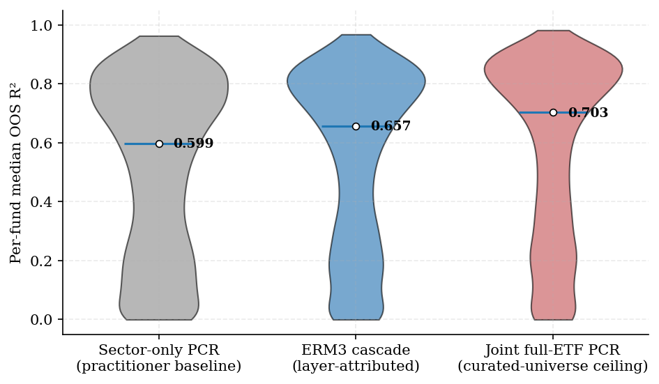
Figure 1. Distribution of fund-level median OOS R² by construction (N = 9,074). Violins show the cross-section; white markers are population medians.
4.2 Paired decomposition
Table 3. Paired OOS R² gaps
| Gap | Median | p25 | p75 | Mean |
|---|---|---|---|---|
| g1 (cascade − sector) | +0.018 | −0.011 | +0.067 | +0.031 |
| g2 (joint − cascade) | +0.027 | −0.008 | +0.071 | +0.030 |
| g3 (joint − sector) | +0.036 | 0.000 | +0.109 | +0.061 |
Means satisfy mean(g3) = mean(g1) + mean(g2). Medians are not additive—reported separately, not a decomposition error.
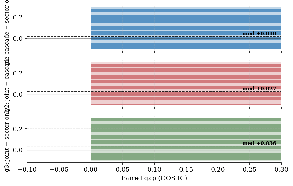
Figure 2. Paired gaps g1, g2, and g3 (stacked horizontal histograms, shared x-axis). Dashed lines mark population medians; values clipped to [−0.10, 0.30] for display.
4.3 Cascade extraction efficiency (primary decomposition metric)
Extraction efficiency (g1/g3, conditional on g3 > 0.01) summarizes how much subsector value a structured estimator recovers on the fit–stability–executability frontier—a metric rarely reported in fund-hedging studies that focus only on absolute R².
Among 6,024 funds (66%) with meaningful L3 value, median efficiency is 0.448; 45% exceed 0.50 and 28% exceed 0.75. Dispersion is wide (p25/p75 = 0.045 / 0.816).
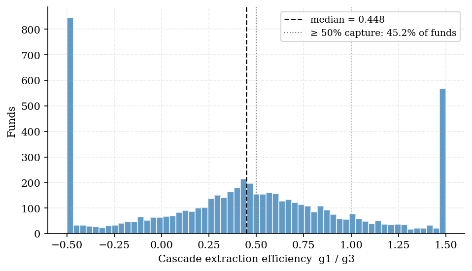
Figure 3. Cascade extraction efficiency (g1/g3) for funds with g3 > 0.01. Display note: values clipped to [−0.5, 1.5] for readability; spikes at boundaries reflect clipping, not winsorization of the underlying census. Median = 0.448 (dashed).
4.4 Conditioning and coefficient stability
Table 4. Median coefficient drift and conditioning (N = 9,649 for conditioning census)
| Construction | Median coef. drift | Median cond. number | Singular rate |
|---|---|---|---|
| Cascade | 0.025 | 2,508 | 0% |
| Joint full-ETF PCR | 0.084 | 156 | 0% |
| Joint OLS (exhibit) | 0.127 | ~48,000* | 100% |
*Where invertible.
Joint PCR never hits singular sentinels but drifts roughly three times as much as the cascade—a key frontier tradeoff for implementers.
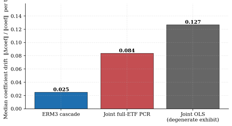
Figure 4. Median coefficient drift by construction (lower is stabler).
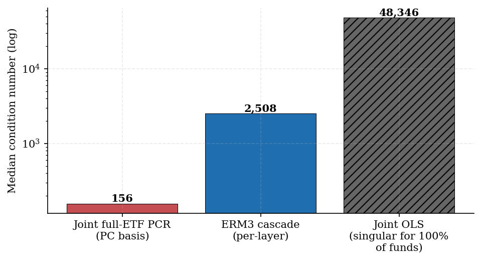
Figure 5. Median design-matrix condition number (log scale). Joint OLS (hatched) is ill-posed for the full sample.
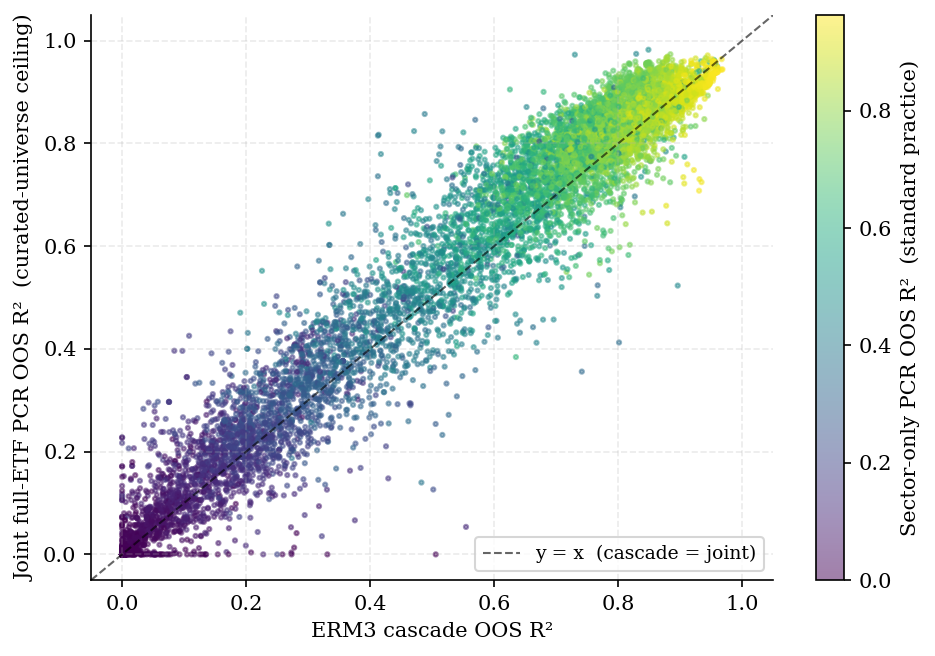
Figure 6. Curated-universe fit ceiling (joint PCR) vs cascade OOS R² by fund. Color encodes sector-only baseline R²; vertical distance above the 45° line is g2.
4.5 Segmentation by L3 marginal value
Table 5 splits the cross-section by total subsector value (g3), a proxy for whether subsector ETFs matter for the fund's hedge. This makes the frontier story concrete for portfolio and risk teams.
Table 5. Results by L3 marginal-value segment (fund-level medians)
| Segment | N | Median sector R² | Median cascade R² | Median joint R² | Median g3 | Median efficiency* |
|---|---|---|---|---|---|---|
| Negligible L3 (g3 ≤ 0.01) | 3,050 | 0.723 | 0.708 | 0.697 | −0.010 | — |
| Moderate L3 (0.01 < g3 ≤ 0.05) | 2,086 | 0.533 | 0.565 | 0.559 | 0.027 | 0.220 |
| Large L3 (g3 > 0.05) | 3,938 | 0.575 | 0.663 | 0.736 | 0.123 | 0.477 |
*Efficiency = g1/g3, defined only when g3 > 0.01.
Funds with negligible L3 value are already sector-spanned—subsector ETFs add little, and the cascade is optional. The large-L3 segment (43% of the sample) is where subsector hedging and cascade value concentrate: median g3 = 0.123 and extraction efficiency ≈ 0.48. Moderate-L3 funds show smaller incremental value and lower efficiency—the frontier bite is largest where g3 is material.
4.6 Robustness to distributional tails
Violin and efficiency plots show heavy tails. We stress-test whether extremes drive headline medians.
Near-zero R². Roughly 3–4% of funds register exactly zero OOS R² in at least one view. Excluding them (n = 8,663) raises gap medians slightly.
High-fit cluster. When sector-only R² ≥ 0.85 and joint R² ≥ 0.90 (n = 474), median g3 ≈ −0.002.
Efficiency tails. Conditional on g3 > 0.01, 18% of funds have efficiency > 1 and 23% < 0. Winsorizing and trimming leave signed conclusions unchanged.
5. Discussion
5.1 Economic magnitude relative to practice
Positive g1 in 63% of funds (p75 = +0.067) is the primary practitioner-facing result. Relative to unregularized sector OLS, the reported gap is conservative.
5.2 Frontier gap to joint fit, not a shrinkage knob
The g2 gap reflects sequential orthogonalization versus joint optimization on the same ETF universe. Closing it requires joint hierarchical estimators with attribution constraints—not incremental peer-mean tweaks.
5.3 Executability versus curated-universe fit
Joint PCR can be decomposed after estimation, but it does not natively produce sequential, layer-controlled hedge notionals. It delivers a single 68-leg basket—adequate for a fit benchmark, awkward for risk reporting and implementation. Coefficient drift 0.084 versus 0.025 for the cascade quantifies the stability leg of the frontier.
5.4 Implication: fund-level view selection
Table 5 supports adaptive view selection: sector-only hedges for the ~34% of funds with negligible L3 value; full cascade where g3 is large. This improves fidelity per implementation dollar without changing the underlying estimators.
5.5 Limitations and extensions
Sample length. N-PORT holdings span ~seven years; evaluations run April 2020–April 2026. Regime stratification is an obvious extension.
Universe definition. The 56 subsector ETFs are an ERM3 curation; overlap among industry funds is not fully stress-tested.
Commercial benchmarks. We do not license Barra or Axioma for fund-level parity.
Holdings-based segments. Table 5 uses g3 buckets; future work should replicate with holdings concentration (top-10 weight, active share).
Causal claims. Results describe predictive hedging fit, not causal attribution of alpha or skill.
6. Conclusion
We provide a paired empirical decomposition of subsector ETF hedging value across 9,074 US mutual funds on the fit–stability–executability frontier. Joint PCR fits better on median OOS R² within our curated 68-ETF universe; the cascade improves materially on sector-only practice and extracts about half of available subsector value where L3 matters (median efficiency ≈ 0.45). That is the cost of interpretability: stable, layer-attributed, executable hedge intelligence rather than the highest-R² black-box basket.
Closing the cascade–joint gap is structural (joint hierarchical shrinkage, constrained joint fit, adaptive view selection). The commercial implication is direct: the product is not selling maximum R² alone—it is selling a defensible point on the frontier that risk teams can report, audit, and trade.
References
- Avellaneda, M. & Lee, J. (2010). Statistical arbitrage in the U.S. equities market. Quantitative Finance 10(7): 761–782.
- Cremers, K. J. M. & Petajisto, A. (2009). How active is your fund manager? A new measure that predicts performance. Review of Financial Studies 22(9): 3329–3365.
- Engle, R. F., Ledoit, O. & Wolf, M. (2019). Large dynamic covariance matrices. Journal of Business & Economic Statistics 37(2): 363–375.
- Fama, E. F. & French, K. R. (1993). Common risk factors in the returns on stocks and bonds. Journal of Financial Economics 33(1): 3–56.
- Fan, J., Liao, Y. & Mincheva, M. (2013). Large covariance estimation by thresholding principal orthogonal complements. Journal of the Royal Statistical Society B 75(4): 603–680.
- Harvey, C. R., Liu, Y. & Zhu, H. (2016). … and the cross-section of expected returns. Review of Financial Studies 29(1): 5–68.
- James, W. & Stein, C. (1961). Estimation with quadratic loss. In Proceedings of the Fourth Berkeley Symposium on Mathematical Statistics and Probability 1: 361–379.
- Jolliffe, I. T. (2002). Principal Component Analysis (2nd ed.). Springer.
- Jorion, P. (1986). Bayes-Stein estimation for portfolio analysis. Journal of Financial and Quantitative Analysis 21(3): 279–292.
- Kelly, B. T., Pruitt, S. & Su, Y. (2019). Characteristics are covariances: a unified model of risk and return. Journal of Financial Economics 134(3): 501–524.
- Ledoit, O. & Wolf, M. (2003). Improved estimation of the covariance matrix of stock returns with an application to portfolio selection. Journal of Empirical Finance 10(5): 603–621.
- Ledoit, O. & Wolf, M. (2004). Honey, I shrunk the sample covariance matrix. Journal of Portfolio Management 30(4): 110–119.
- Lettau, M. & Pelger, M. (2020). Estimating latent asset-pricing factors. Journal of Econometrics 218(1): 1–31.
- López de Prado, M. (2014). The deflated Sharpe ratio: Correcting for selection bias, backtest overfitting, and non-normality. Journal of Portfolio Management 40(5): 94–107.
- López de Prado, M. (2016). Building diversified portfolios that outperform out of sample. Journal of Portfolio Management 42(4): 59–69.
- Stock, J. H. & Watson, M. W. (2002). Forecasting using principal components from a large number of predictors. Journal of the American Statistical Association 97(460): 1167–1179.
- Vasicek, O. A. (1973). A note on using cross-sectional information in Bayesian estimation of security betas. Journal of Finance 28(5): 1233–1239.
Appendix A — Replication
On request we provide: (i) paired per-fund summary statistics (N = 9,074); (ii) aggregated cross-sectional distributions for Tables 2–5 and Figures 1–6; and (iii) figure-generation code. Contact conrad@bwmacro.com.
Working paper · Not peer-reviewed · Version 2026-05-24 · Data as of 2026-04-30 month-end evaluations · riskmodels.org/research/cascade-hedging
Footnotes
-
Vasicek shrinkage (brief). At each layer, each stock's factor beta is shrunk toward the cross-sectional peer mean for stocks assigned to the same factor leg. Shrinkage intensity is tuned with an out-of-sample gate (applied at L2 and L3 in production; L1 left unshrunk). ↩